Database
Window Help File
Contents:
Adjusting program start-up behavior
Viewing molecules and reactions in a database (including with ChemSite)
Creating databases of mixtures and reactions
Adding records (molecules)
Editing records (values for a molecule)
Adding fields (properties)
|
Menu Descriptions |
|
|
Edit (continued from left column bottom) |
|
|
- Fields (Properties) |
|
|
- Open |
|
|
-- MDL SD Files |
|
|
- Find |
|
|
- Sort |
|
|
-- XML files |
|
|
- Subset |
|
|
- Save |
|
|
-- MDL SD Files |
|
|
-- XML files |
- XY Plot |
|
-- HTML files |
- 3-D Plot |
|
-- EXCEL |
Analysis |
|
|
|
|
- Close |
|
|
- Copy |
|
|
- Paste |
|
|
- Records (Molecules) |
|
|
|
|
|
|
|
|
|
|
|
|
|
|
|
When you first install Molecular Modeling Pro, you set two options that control the behavior of the program when you start it up. You can always go back and change these two options by selecting "Initialize Links" from the File menu of the Drawing window. There are four possible combinations of these two options:
- Open in drawing mode with no default database file specified. The program opens with the drawing window open and the database window closed and no database file open. You can open the database of your choosing by selecting "Open database" from the File menu. This is the program's default.
- Open in drawing mode with a default database file specified. The program opens with the drawing window open and the database window closed and no database file open. However, choosing Open database from the File window will automatically load the specified database
- Open in database mode with no default database file specified. The program opens the drawing window and will prompt you for the file format and the name of the database file to open.
- Open in database mode with a default database file specified. The program opens the drawing window and opens the database window with the default database displayed.
Creating Databases
Creation of databases will be a familiar task for past users of Molecular Modeling Pro. It is still done from the file menu (Save Database) of the Drawing window. However, underlying the similarity of appearance are many changes and additions that make the program more powerful, flexible and consistent.
Saving the drawn molecule(s) to a database: Draw in the molecule or molecules. Then, while still in the Drawing window, choose the File menu, then Save Database, and then choose Save this molecule to the database.
If you have only drawn one molecule: The program will first ask you for the data base name. You have a choice of four file formats at this point:
- ACCESS
You will probably not be able to save data to an
ACCESS data base created by some other program from the Save Database feature
of the DRAWING window (unless your fields have the same data types as expected
by MMP for fields with the same name - MMP uses the memo, text and single data
types from ACCESS 97). You may view and modify such databases from the DATABASE
window (MMP will use the data types contained in the existing database). You
can then save the data to a different file name and MMP will create an MMP
style ACCESS database from the database created with another program. Note if
you open an ACCESS database created with another program that contains multiple
tables, only the data in the table you open will be saved in the MMP ACCESS
database. Versions supported by MMP are
ACCESS 95 (3.5.1 Jet), ACCESS 97 and ACCESS 2000. Saving will convert an ACCESS 2000 database
to ACCESS 97. Technical Information: Opening ACCESS this way uses Microsoft
You can also open ACCESS databases as "read
only". You cannot modify data if
you open it this way. The advantage of
this is that large databases open much faster.
If the database is not yours, the owner may prefer you open it this
way. Technical
information: Opening it this way uses Microsoft
WARNING: Saving a database containing more than 7 text
fields will lose data in text format. Furthermore it may cause the database to
be unreadable if the text field contains commas as MMP will place it in a
numeric field location and when read back in, the commas will be seen as field
delimiters! If you are not going to use
- MDL SD File. This text file
format is the industry standard for transporting chemical data between
otherwise incompatible programs. It is not particularly efficient at file
input and output, but is not significantly worse than
- Tab-delimited text files. Another industry standard format. These files, for instance, can be read, as is, directly into EXCEL.
- XML and comma separated value
text files can also be created with MMP, but these file types are created
by first creating a database in one of the above four formats. Then open
the database and save in XML or
Next the program will ask for the name of the file to save the structural information.
If you are saving to an ACCESS database you have the choice of saving the
structural data internally in the .mdb file (by
selecting the same file name that you chose for the database file), or saving
to an external connection table file. If you are saving to an
The file formats for external connection tables are:
- MACROMODEL files. A format
invented at
- MDL Molfile. The most widely used connection table format in the business. Almost any chemistry program, now days, reads this file format. There are several versions of the format, though, and it is not always applied uniformly. MMP overwrites any existing file with the name you choose for the connection table file with the structure currently depicted on the screen.
- Brookhaven pdb file. This file format contains a lot of information that no other file format contains. MMP reads this format, but does not faithfully reproduce the non-structural information contained in them. For this reason, if you request this file type and a file already exists with the name you select, MMP will not overwrite the file. For all other file types, MMP does overwrite the file (if you have a file called temp.dat with benzene in it and wish to store benzimidazole to temp.dat, we need to overwrite the file). Note that you can create pdb files with the residue information with the companion program ChemSite.
- MMP/
Next you will be asked to choose the calculated fields to save. Note there
is a check box in the lower right part of the screen that allows you to check
off most of the properties. The properties not checked off are the ones that
require interaction between the user and the program and the properties
calculated by
If you chose to save to an ACCESS data base, the program next will ask you if you would like to create some additional fields for experimental or literature values. This would be a good time to say yes if you plan to add some of your own data to the data base. Fields can be added later, but it is easiest to do it now.
At this point, you will be asked if you want to view the data base. If yes,
it will open up in the data base window, where you can further edit it or view
the data and structures it contains. Or you can say no, and proceed with adding
more molecules from the Drawing window. Note that there is a major difference
between adding molecules from the Drawing window and the Database window:
Saving from the drawing window saves directly to the data base causing a
permanent addition there. Adding a molecule in the Database window only adds it
to the database kept in temporary memory. You must Save the database for the
change to become permanent (similar to how the program
Note on Adding more records to the database from the Drawing window: You can add more molecules to the data base using the same menus. MMP will no longer give you the option of saving structures internally or externally, but will figure out what you did before and do the same again. The same applies to saving mixtures and reactions as one record or multiple records (see below). If you wish to create a data base of mixtures or reactions with each molecule stored as a separate record (with its own properties) that also contains some individual molecules, create the data base with a mixture or reaction, not a single molecule. Otherwise, on subequent additions to the database, MMP will save everything to a single record.
Creating databases of mixtures and reactions - if you have drawn more than one molecule:
Read over the information above for saving single molecules, for it all still applies.
When creating a new database, In addition, you have a decision to make on how to store the mixture and reaction information. When the program asks you if you want to store the molecules in a reaction or mixture:
- If you say yes, the program
will store each molecule as a separate record. It will create additional
molecular properties to store: molar ratios, component type (starting
material, intermediate, product, mixture), reaction conditions
(information above and below reaction arrows), the weight of each material
added, the solvent volume, the trade names of each molecule, their
manufacturer and
Choosing yes has the added advantage of being able to reproduce the reaction drawings from the MMP Database window. Check the View molecules as mixture or reaction menu item in the Options menu.
- If you say no, the program
will save all the molecules to a single record. The connection table will
contain information for all of the molecules. No fields describing molar ratios,
reaction component types or reaction conditions will be stored. However,
if you choose to store the connection tables to the MMP/
Editing Records (Molecules): Just type the new values into the spreadsheet or the file card text boxes. The changes do not become permanent until you save the data.
Note that the column width of the spreadsheet column can be changed. Click down on the place at the top of the spreadsheet between two field names and drag the column margin to the desired location.
Viewing Molecules and Reactions in a data base:
Special note: Double clicking on any line will display and load the structure into the MMP drawing window. Some of the viewing options, listed below will cause MMP to update the drawing window automatically (which will cause the molecule currently displayed to vanish).
Reactions: Two types of databases can display
reactions. One is a database created with MMP 5 when you have chosen to say yes
to the question "do you want to save the molecules to a mixture or
reaction?" The second is an MMP/
The File Menu
Open - opens a data base file
Use the standard field names with these files to make life simpler. Here are some of the standard names:
|
Standard Name |
What it is (type) |
|
Name |
Chemical name (memo field) |
|
Smiles |
Smiles Notation (memo field) |
|
|
|
|
ID |
Index number (32 bit integer - in VB this is type "long") |
|
Connection_Table_Name |
Connection table file name (memo field) |
|
Chemistry |
An MDL Molfile embedded as text in the data base (memo) |
|
Information |
A memo field containing information about the molecule |
|
Formula |
Molecular formula (e.g. butane = C4 H10)(char * 256) |
|
Molecular_weight |
Molecular weight (single, floating point) |
|
Molecular_volume |
Volume contained in spheres of Van der waal's radius |
|
Log_Kow |
Log 10 of the water/octanol partition coefficient |
|
Boiling_Point |
Boiling point in degrees C |
|
Etc. |
|
A complete list can be found in the file "fldnames.txt".
Note that there are two ways to store connection tables (as a separate file or as text in the database). For most uses we recommend separate files. Performance will be somewhat faster with text in the database, but out of memory errors will also be more frequent. The exception to this is when using the Microsoft ACCESS data format, when storing the molecular structures as memo fields in the databases should be well handled.
Formats supported:
Molecular Analysis Pro .csv text file.
This file format can be used with Molecular Analysis Pro. It has its own
peculiar structure. The first line is a header that tells the programs what
type of data the numeric fields have (e.g. molecular weight = 1). The second
line has the field names. Each subsequent line has the data for one record. The
format of the file is comma-separated value ASCII text. This file format always
stores 80 fields, no more, no less. The first seven fields are string fields up
to 64kb in length. The next 72 fields are single precision floating point
numbers (can contain integers too). This format always stores the molecules as
separate files and stores the name of the connection table file in the last
field of each record. Numerous unused fields are typically found in
Microsoft ACCESS databases (.mdb). This is the most versatile format for use with Molecular Modeling Pro as it gives you features not available with other formats. Be careful with using this format with data bases shared with other people, as the changes you make will become permanent after you save the data or hit the Update button. The extra features available with this format area a result of the fact that the Microsoft Jet Engine Relational Data Base software underlies all that happens in MMP when using this format. Performance with large databases will be best using this format. There is also an opportunity for those who know SQL, to directly interact with the database in an almost unlimited fashion. (See the SQL editor in the Edit menu, described below). Use of SQL is the only way to add new fields using this format.
MDL SD File. Standard chemical text format used for exchanging data between otherwise incompatible programs. It is not recommended to use this as your standard data storage format. Performance with databases containing large numbers of molecules or very large molecules will be problematical. For instance, MMP will set aside 64 KB for every structure in the database, which may quickly run your computer out of memory. However, you are welcome to try it out. On smaller databases, with smaller (<150 atoms) molecules there should be no problem. Note that the SD Files include the Molfiles (structural connection table) for all of the molecules in the database.
Tab delimited text files that can be input by most any program: This is the standard text format used by EXCEL and many other programs. MMP expects the first line to contain the field names and each subsequent line to contain one record.
Comma separated values text (.csv). This is the alternative way of saving text files (to tab-delimitation), that has been used by some programs. Again, MMP expects the first line to be the field's names and each subsequent line to be a record (one molecule with data). It is recommended to use the option of storing each molecule in its own file with the file name being included in the .csv file.
XML
files: (aka Extensible Mark-up Language). Microsoft and others are pushing this
format as the internet standard for data base transfer. MMP reads and writes to
these files. MMP uses the
MMP molecular fragment files (.ssf). MMP creates these files as keys for the substructure searches, but they may be quite useful for building methods for calculating physical properties from structure. They contain information on the fragments and atom types for each molecule. For instance, typical fields include the number of carbons in aromatic rings, the number of amide groups, the number of N-N groups, etc. To create this file for a database, run a substructure search. Do not add new things to this database, as MMP will automatically update it when you add new molecules.
Paste tab-delimited text from the Clipboard: This is a way to get data from EXCEL or other programs which copy data to the clipboard as tab-delimited text. Select the area in EXCEL containing the field names and all the data. Copy it to the clipboard. Then paste the data into MMP. MMP expects the first row it encounters to contain the field names and each subsequent row to contain a record (one molecule). Combined with MMP's Save/Excel option this procedure allows you to easily add new fields to a data base, or manipulate the column order or rename fields.
Connect Directly to a large ACCESS database: MMP also supports a direct connection to ACCESS databases. When connected directly to the database, changes made will change the underlying database (no Save is necessary). This method is intended for connections to really large databases since not all of the data need be read into memory for this to work. It also has the advantage of allowing you to get to databases with complicated multi-table structure and save changes and add new records to that database. Some limitations have been built into this method, though, to limit the damage that can be done to the database. These limitations are that you cannot delete records, add fields, sort, or subset the data. Nor can you save the data to an Microsoft ACCESS database (this is to prevent overwriting the database). Again you will not have to save the data to save changes as this is done automatically after you move to a new cell in the spreadsheet.
Save - saves the data base with changes
Molecular Analysis Pro .csv text file. A description of this file type is under Open above. Use this file type when you expect to analyze the data with Molecular Analysis Pro
Microsoft ACCESS database (.mdb). This is the best general-purpose data base format supported by MMP. For a description see the Open method above. Note that at present, no other program except MMP will read the structural Molfiles embedded in the database as structures. When passing structures and data to other chemical programs, the MDL SD File may be your only choice.
MDL SD File. Standard chemical text format for exchanging data between otherwise incompatible programs. Not recommended as a general-purpose database file format.
Tab delimited text file that can be input by most any program. This is the standard form that EXCEL and the clipboard use for passing tables of data.
Comma separated values text (.csv). This is another standard format for passing data between MMP and many other programs.
XML files (.xml) for later use in HTML pages. These files can be used to paste XML tables into HTML documents. MMP also opens this data type, so you could use this as a means of storing the MMP data bases. Note, as of 2002, this file format is still rather new, and not all browsers support XML.
HTML files (.htm) creates an html page with a data table that can be viewed with a browser or amended further by another program. After selecting this item the user is asked to do the following:
- Type in a title for the page which will be supplied above the database.
- Choose which records (compounds) to include in the table. Note there is a check box at the bottom that allows you to choose all of the records. Selecting the check box again will deselect everything.
- Choose which fields (compound properties) to include in the table. It may be best to leave out fields as the page width can become cumbersome and the page not particularly good-looking if too wide. Almost always you will want to include the compound name.
- Choose whether to save the structures as JPEG files linked to the HTML table. Any work you have displayed on the Drawing window should be saved before running the HTML creation routine (if you want to keep it), as otherwise it will be overwritten during the creation of the JPEG files.
The program will then create one or several HTML pages automatically. It creates a new page for every 25 records (compounds). If there is more than one page, it automatically adds page navigation buttons (Next page, Previous) just above the table, so you can access one page from another.
If you choose to save the structures as JPEG files, then separate JPEG files for each molecule will be saved to a subdirectory called /moldir and the URL will be linked to the HTML data table via the first column of the table. When you place the HTML data tables on the server you must create this subdirectory (call it moldir) on the server too and copy all of these JPEG files to that subdirectory. Use lower case letters as MMP saves all internet files lower case to be compatible with UNIX servers.
When saving the structures choose the background color from the Drawing window's Format menu. Likewise choose to have perspective on or off, choose the display type (from the Display menu), and choose whether labels are on and off. Do all of this before running the HTML page creation routine. One of the better ways to show the structure clearly is to choose the wire frame display with Perspective on and Labels on. Also turning on dot surface (density 4), molecule outline and wire frame (all concurrently) with Perspective off and Labels on can give a nice view. If you wish solid spheres, the best display is dot surface with density set to 1. Solid spheres, though, obscure some of the atoms from view and do not work well with atom labels. The molecule pictures are automatically cropped to give a smaller sized (and faster loading) JPEG file. You can control the size of the drawing somewhat by using the Scale button in the drawing window.
EXCEL - opens EXCEL with the current data displayed. Note that to actually save the data, you must do this with EXCEL
Copy tab-delimited text: This places the entire data base on the clipboard where it can be copied into any program that supports this format. The first line is the field names and each subequent line is one molecule (record). The fields in the records are separated by the tab character and the end of the line is a single line feed character (ASCII character 10).
-- Print current Record (molecule): Prints out all the values for the currently selected molecule, one line per field to a text editor. From there the user can enhance the appearance and print out the data.
-- Print 1-3 fields for all molecules - Prints out the molecule names and 1-3 additional fields selected by the user to a text editior. From there the user can enhance the appearance and print out the data.
Close - Closes the data window. MMP remains open, with the Drawing window still there.
The Edit Menu
Copy - Copies the data in the cell selected in the spread sheet to the clipboard. To copy an entire database, use the File/Open/Copy database to clipboard menu items instead of this one.
Paste - Copies the data on the clipboard into the current cell in the spread sheet. To paste an entire database use the File/Save/Paste database menu item instead of this one.
Records (molecules)
-- Add a molecule: The molecule currently displayed in the drawing window will be automatically added to the record set in memory. Note that it does not become a permanent part of the data base until you have saved the data base. The structure will be saved if the data base saves structures to connection table files. All recognizable calculated fields will be given values. There must be a recognizable chemical structure associated with the record, or MMP will be unable to calculate any physical properties.
Remember that if you have specified interatomic distances, angles, dihedral angles, sterimol parameters or Hammett sigma values, they require user input on the Drawing Window. If the data base appears to have gone away and the program is just sitting there, it may be awaiting your input on the Drawing Window.
Note that there is a second way of adding a record. At the bottom of the spreadsheet is a row with an asterisk at the left. Typing in data in this row, then moving to a different row will cause a new record to be made. Make sure you add the structure to the appropriate column. If the structural field contains embedded Molfiles, you may copy a Molfile from the clipboard (e.g. from ChemSite) into the column containing the structural information. If the structural field contains connection table file names, then put the file name in the column instead. After inserting the structure and moving to a different row, move back to the newly created row to calculate the fields that MMP calculates. Do this with the Update molecule's fields menu item.
IMPORTANT NOTE: You can also save molecules to the database from the Drawing window. This works in a totally different way and can get one into a little trouble. For instance, if you have not saved data typed into the spreadsheet and then use the Drawing window's data base save method, it will write the new record directly to the data base saved on disk. If you then open this data base, the changes made in the spreadsheet will be lost. Conversely, if you don't open it, then save the changes made in the spreadsheet to the data base, the new molecule added will be lost. In other words, save your work on the spreadsheet before adding a new molecule with the menu on the drawing window.
-- Delete a molecule; Deletes a molecule from the record set in memory. This change does not become permanent until the data base is saved. The molecule deleted is the one currently selected.
-- Update molecule's calculated fields: This will recalculate all the fields that MMP recognizes with the latest algorithms of MMP. This is included to give consistency to data bases created years ago or with a different tool. MMP recognizes fields based on their field names. To see the list of field names that MMP recognizes, examine the file fldnames.txt. Note that the changes do not become permanent until you save the data base.
-- Replace with the current molecule drawn. This will replace the molecule in the selected row and its associated calculated properties with the structure and calculated properties of the molecule displayed in the drawing window.
Fields (Properties)
- Add Field (property). See the description later in this document.
-- Update a properties's values for all records: This will recalculate the values of one field for all the molecules in the data base. This is included to give consistency to data bases created years ago or with a different tool. MMP recognizes fields based on their field names. To see a list of field names that MMP recognizes, examine the file fldnames.txt. Changes do not become permanent until you save the data base.
-- Restore or Update a field from an ACCESS database. This feature only will update a field using data from a Microsoft ACCESS database. You will be asked to select one or more fields. The program will replace the data in your current database with the data from the selected ACCESS database. Text field replacements will only be made when the text in the current database is shorter in length than the text in the archived ACCESS database. For numeric fields: as long as the data in the archived ACCESS database is not null (missing), all numbers in the existing database will be replaced by the data from the archived database.
Find - Finds a string of text or numbers anywhere in the spreadsheet.
Sort - Sorts all rows by the currently selected column from low to high. Note that you should click on a column in the spreadsheet before selecting Sort from the menu.
Update All Calculated Properties for all molecules - This updates every calculated field for every molecule (record) in the database. It updates molecular formula and SMILES notation as well as all the calculated numeric fields. You might want to do this for two reasons:
1. Create new fields with names that MMP recognizes as calculated properties. Fill them automatically with this option.
2. Over time, methods for calculating properties with MMP have changed. For instance, the old methods of calculating water solubility and the solubility parameters have been replaced. To make current calculations consistent with older calculation in existing databases, update the old database with this option.
WARNING: MMP knows which fields to update by their name. If you have named a field of literature values or experimental values with the same name that MMP gives to a calculated field, then it will replace these values too, and if you save the changes, the data previously there will be overwritten! Rename these fields before using this routine so they won't be overwritten. To change the name of a field, use ACCESS or EXCEL or some other program that reads in one of the formats supported by MMP (for instance in tab-delimited text format). If you have an ACCESS reaction database and don't use ACCESS to modify the name, be careful not to close MMP while you do this if you have a reaction database, as you will want to keep the reaction table when you read the database back in. For a list of the field names that MMP recognizes as calculated fields see the file fldnames.txt
Databases containing large molecules and
Substructure Search - Draw in the substructure that you wish to use for the search. Then select this off the Edit menu of the data base window. If there is no keys file for the database, then one will be created and this can take some time. The keys file contains lots of structural information on all the molecules in the database. Once it is created, subsequent searches will be quite fast, even on large databases. The keys file has the same file name as the data base, except that it has the file extension .ssf. An option to do a more exhaustive search after the key search is given, but this is usually not needed.
After you have selected Substructure Search from the Edit menu the program will ask you if you want to create a dataset of the molecules containing the subset. Usually you will want to choose NO here, especially if you have made changes to the database and not saved them. Choosing YES will create a new database containing only the molecules containing the substructure (which you can make permanent by saving). Choosing NO will give you a list of molecules which contain the substructure from which you can select molecules in the current database.
If you choose to create the subsetted dataset: The Records will be modified with the structures found. Take care to saving this data, as the records not in the subset will be deleted, if you use the same file name to save to.
After running the substructure search a new menu item will appear on the Edit window entitled "Restore after substructure search. This will restore the database to how it was before the restoration including any subsetting done prior to the substructure search.
Subset - This is accomplished with the Active X Data Objects Filter command, so the record set is not actually altered. Changing the subset criteria to a more generous span will retrieve records made "invisible" by a previous subset. Saves made after subsetting will apply to the saved data base, so you may want to give the saved database a new file name.
After running the subset a new menu item will appear entitled "Restore after subset". Running this routine will restore the database to how it was before the last subset was done.
The View Menu
Note that memo sized text cannot always be viewed easily in the
spreadsheet or even in the file card text boxes. To see them, select the page
and click on the gray line at the bottom of the Database window. This will
display the text over the entire database window. Click on the text again and
the gray line will return to its normal size.
SpreadSheet - Displays the data base in a spreadsheet format. To display the molecule, double click on its row in the spreadsheet.
Structure in Drawing Window - Resizes the drawing windows so that the left most column is displayed (usually the compound name field). If you resize the database window to see more columns, the drawing window will also automatically be resized. Hitting the < and > buttons at the lower corners of the database screen or the right or left arrow keys will scroll through the pictures of the molecules. Clicking on the name of a molecule will cause that molecule to be drawn in the drawing window.
Selected Molecule with Chemsite - Again, the database window will be resized so that the left most column is displayed. ChemSite will be automatically loaded if MMP can find it. If MMP does not find it, you will have to start ChemSite manually. Place the Chemsite window where you want it and size it to taste. ChemSite will subsequently remember where you placed it and its size. Selecting a molecule from the spreadsheet will place a molfile on the clipboard that will be picked up by CHEMSITE. Note that this requires version 3 or better of CHEMSITE. Single clicking on a compound name brings the CHEMSITE window to the front with the molecule drawn.
File Card - Displays the data for the selected molecule or record in a more readable format, by placing a file card containing its data over the spreadsheet. Supports a maximum of 237 fields.
Reaction Table - This will display the reaction conditions that appear above and below the reaction arrows and allow you to edit them, as well as the solvent volume used in the reaction. It also contains the file name used by the next menu item "Edit Reaction Description." Going to this view will not lose any information in the main data table. If you save after going to this view, the changes made in the main table will still be remembered and stored. This menu item is only available to ACCESS data bases containing a reaction_table.
Edit Reaction Description- This allows you to store a full description of the reaction, molecule or mixture in rtf (rich text format), Microsoft WORD or text format. You can store pictures in the rtf format. MMP uses the WordPad application to display the file. You can drag and drop items into the document. The document will remember and will display formatting such as several fonts in the same document, underlining and bold fonts. You can create this document with a different program, then tie it to the MMP database (this file name goes into a field in the reaction table). This menu item is only available to ACCESS data bases containing a reaction table. Remember to Save your work before exiting WordPad. Use the Save function from the File menu and not Save As. You want the name of the file to be the same as the one stored in MMP's Reaction table.
The Graphics
Menu
Simple XY Plot - draws an x-y plot of two fields selected off a menu in a separate window. Two different graphics windows alternately display the plots, so that two plots can be viewed simultaneously and compared. The regresion statistics are displayed in a separate window usually located near the bottom of the screen. Double clicking on a data point reveals the point's identity (an advantage over the Advanced Plot).
Advanced XY Plot
There are lots of options available to the user for drawing X-Y plots. The user chooses one X axis parameter and as many Y axis parameters as he wants. A separate line or curve and set of data points is drawn for each Y axis parameter. From an artistic stand-point the user should be aware that their are only 15 different colors for use in differentiating the Y axis to the screen, and only 4 different line types and 8 point symbols for printing. Your graph will look crowded if you put too many Y axes on the chart. After the X and Y axis parameters have been chosen, an options panel appears. Here is a description of the options:
a) Draw best fit regression line: This option will perform a simple regression of x on y if the data is not transformed, and will draw a regression line through the points. If a polynomial model is chosen, then the program will draw the curve described by the regression equation. If the data has been transformed, then the model will draw a curve if the axes are not transformed, and will draw the regression line described by the regression equation if the transformation is applied to the axes.
b) Join points, sorted by x: This option does three things. First, the data is sorted by the x axis from low to high, so trends can be observed. Second, lines are drawn between the individual data points, so they appear joined. Third, the polynomials options are turned off, and any transformation selected will be applied to the axes, as well as the points. The program will not draw a regression line or curve if this option is selected. The sort is not applied to the data base, only to the graph.
c) Join points without sorting: Does the same as b above, but without sorting. This allows the user to sort the data base by a third variable (from the file card screen).
d) Draw data points: Checking this box will cause the individual data points to be displayed. Otherwise only the line or curve will be drawn. If boxes a,b and c above are not checked the data will be displayed as a scatter plot of points.
e) Calculate means of y by x. Values of y are expressed as mean y for each value of x, with an error bar representing one standard deviation.
f) Divide y by block variable. Separate lines or curves are drawn for each separate value of some third block variable. For instance with the following data:
Name X Y Z
methane 1 2.5 1
ethane 2 3.7 1
propane 3 4 1
n-butane 4 4.2 1
ethene 2 5 2
propene 3 6.4 2
2-butene 4 8 2
Two separate lines of X-Y values would be drawn for the two values of Z.
g) Print graph automatically. Checking this item results in the graph being printed out. Usually graphs printed out by this option look better than bit mapped screen prints, but are in black and white. Do a screen print for color output after the plot is drawn.
h) Color points by a third variable. The data points are colored by a third parameter selected by the user. For black and white print outs the data points have different symbols.
i) Make points numbers. The data points are displayed as numbers instead of circles or other symbols. The compounds corresponding to the numbers are listed in a legend below the graph.
j) Make all y axes the same scale. If this option is selected then the minimum and maximum y values selected by the user, or if not selected, the minimum and maximum y values of all the y axis parameters will be used to scale the y axis. If this item is not checked each y axis parameter will be scaled separately by its minimum and maximum y value. Check this box when all the y parameters are in the same units. When comparing apples and oranges don't check this box.
k) Show residual plot. The plot of predicted versus residual values for the regression models of the first y axis parameter can be observed after the X-Y plot is shown.
l) Minimum and maximum x; Minimum and Maximum y. Typing in values in these boxes has two consequences. First the x and y axis values can be set by the user with this option. Furthermore, any x or y values outside the values typed in will be excluded from the regression analysis and the graph. Thus, this is a way of subsetting the data, without effecting the data values associated with the file cards.
m) Calculate area under the line. The area under the curve or line will be calculated and appear in the messages window below the graphics window. The messages window also will contain the regression model and some statistics.
Transforms:
n) Polynomials of x: Checking these terms adds squared, cubed and fourth power of x to the regression models. For instance, checking 3 results in the model : y = b(0) + b(1)*x + b(2)*x^2 + b(3)*x^3
o) Log(y) or Log(x): Transforms y or x by its natural logarithm. If y or x are less than or equal to 0 the value is set to missing.
p) 1/y or 1/x: Transforms y or x to its inverse. If y or x equal zero then the value of y or x is set to missing.
q) logit of y or logit of x: Transforms y or x by: log(y/[maximum y-y]). Missing values are generated if maximum y-y = 0 or y/[maximum y-y] <=0.
r) binomial of y or binomial of x: Y or X are transformed by y = arcsin(sqr(y)). Missing values are generated when y <0.
s) Show all transforms: Checking this causes the program to calculate the regression models for several transforms and display them on the graph and in the messages window. Models considered include: untransformed, log(y), log(x), log(y) and log(x), 1/y, 1/y and 1/x (double reciprocal plot), logit(y), binomial(y).
t) Transform axes: If this box is checked the transformations will be applied to the axes and the X-Y plots will be lines (unless polynomial models are also selected). Otherwise, the axes will be untransformed and log, logit, inverse and binomial models will be drawn as curves.
Title: Type in a title to appear above the graph here.
Legend: Type in a legend to appear below the graph here.
Font Options:
u) Fonts. Click on the font name in the list to change the screen font.
v) Foreground and Background: The colors of the graph foreground (text) and background can be changed with these buttons.
w) Line thickness: The lines in the plot can be changed too. "1" is the default, and the thinnest line possible.
x) Font size: This changes the size of the font. 8.25 is the default.
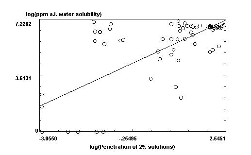
log(ppm a.i. water solubility) =
4.69128784326029
+ .992016058970828 * log(Penetration of 2% solutions)
r squared = .522832786187381, n = 64, probability = 1.50524410603549E-11
This is an example of the x-y regression plot drawn by Molecular Analysis Pro.
3-D Graph
Select the response (y axis) variable and the two causal variables for the plot. Causal variable 1 will be the x axis, and variable 2 will be the z axis. An options panel will then appear. Here is the list of options:
a) Print output to printer: automatically prints out the plot. The appearance of this plot is usually better than a screen print (which is the alternative way of printing out the plot), but will be black and white. Use the Screen print method for color plots.
b) Use square of causals. The model used is y = b(0) + b(1)*x1 + b(2)*x1^2 + b(3)*x2 + b(4)*x2^2.
c) Use cube of causals. Adds the cubed causal terms to the model.
d) Transformations: The response and causal variables can be transformed by the natural logarithm (log(y)), the inverse (1/y), log inverse (log(1/y)), logistic transform or binomial transform by checking the appropriate box.
e) Response and causal minimum and maximum values. The minimum and maximum values of the x, y and z axes are set with these typed in values Any values falling outside these ranges are not excluded from the analysis (unlike the X-Y plot above). The default values are the minimum and maximum values found in the data base.
f) Background and Foreground (text) buttons set
the background and text colors to be used in the plot.
The program then does a multiple regression analysis to determine the contours. The following additional parameters are used in the regression analysis:
if n > 8 then the causal parameters are multiplied by each other if n>16 then, in addition the square of the two causal parameters are included in the model;
if n>24 then the cubes of the two causal parameters are included in the model.
After the calculations are complete, the user is given the chance to view the statistics underlying the model, to see if the underlying model is any good. The analysis of variance and the statistics for each individual parameter are given first. A good model will have a high r square value, low model standard deviation, high probability and high F value. The F values for each individual causal parameter should be significant (probability <0.05). These criteria may not always be met, though, even with models which have good predictability. The parameters used here are often approximations for much more complex
causal effects.
Next the program will allow the user to:
1. Print the statistics to a file
2. View a table of observed, predicted and residual values
3. Plot the observed versus predicted values (this is a regression plot as described under Graph/Regression plot). This plot should be highly correlated with uniform variance.
4. Plot the predicted versus residual values. The points in this plot should ideally be a random scatter plot.
The program then will generate the 3-D line plot (see example below).
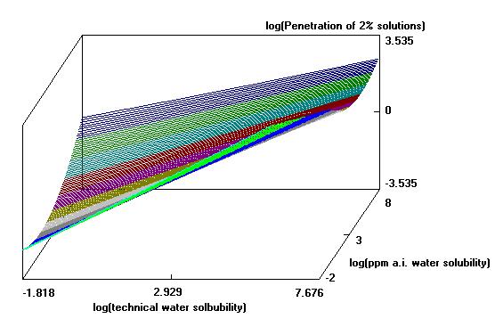
Example of a three-D line plot...
Contour plot
This program will plot out a contour plot of two causal variables colored as a value of a result. The user selects the result and two causal variables from parameter lists. The options panel described above under the discussion of the 3-D line plot then appears. The program then does a multiple regression analysis to determine the contours. The following additional parameters are used in the regression analysis:
if n > 8 then the causal parameters are multiplied by each other if n>16 then, in addition the square of the two causal parameters are included in the model; if n>24 then the cubes of the two causal parameters are included in the model.
After the calculations are complete, the user is given the chance to view the statistics underlying the model, to see if the underlying model is any good. The analysis of variance and the statistics for each individual parameter are given first. A good model will have a high r square value, low model standard deviation, high probability and high F value. The F values for each individual causal parameter should be significant (probability <0.05). These criteria may not always be met, though, even with models which have good predictability. The parameters used here are often approximations for much more complex causal effects.
Next the program will allow the user to:
1. Print the statistics to a file
2. View a table of observed, predicted and residual values
3. Plot the observed versus predicted values (this is a regression plot as described under Graph/Regression plot). This plot should be highly correlated with uniform variance.
4. Plot the predicted versus residual values. The points in this plot should ideally be a random scatter plot.
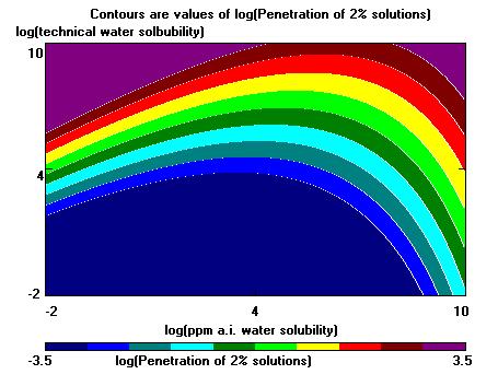
Example of contour plot...
Next the program will draw the contour plot. The colors (unless black and white) will go through the colors of the spectrum (violet = lowest result, blue next, green next, yellow next, dark red = highest result). If the user has selected black and white, then instead, the highest value result is colored white, and other values are black, separated by white lines. To print out the contour plot select File/Print Graphics Window/destination (printer, clipboard, .BMP file) while the contour map is on the screen. A message box will appear when the drawing ends listing the compounds in the data base with highest predicted result.
Rotatable 3-D Plot - a rotatable 3-D plot of the points for three fields is generated. Selecting menu items from the Rotate menu in the Graphics window initiates rotations. Holding down the left mouse button will temporarily stop the rotations. This plot can be valuable for looking for clusters of data. Planes indicate linear relationships between 2 of the variables. Lines indicate relationships between all three variables.
The Analysis
Menu
Molecular Modeling Pro Plus has two methods for automated generation of QSAR/QSPR models which were designed to let chemists with only a general knowledge of statistics create usable models fairly quickly. You access these methods by first opening a database. You must first add the experimental data you wish to model to the database by typing it in or importing it from Excel. Then you just select either "Substructure Analysis" or "Stepwise regression" from the Analyze menu of the Database window. The Substructure Analysis routine will analyze all the molecules in your database for the unique sub-structures contained in the structures and make variables from the molecular fragments to correlate (regress) against the experimental data. The Stepwise regression model will use all the existing fields (calculated and experimental properties) already contained in the database instead of sub-structural fragments. A further explanation follows.
1. Substructure Analysis.
To access this feature: Open a database. Go to the Analyze menu. Choose the first item, "Substructure Analysis."
What this analysis will do: After you choose the property to model, this method will analyze all the structures in your database and create independent variables of the substructures contained within the molecules. It will then use Stepwise multiple regression to find the substructual features that are significantly correlated with the property and places the model in your \models subdirectory. You can then predict the property of any molecule you draw from the Drawing window by selecting "user defined properties" from the Calculate window.
What can be analyzed: This method does not care what atom types you have in your database. It creates the substructures from the molecules themselves, not from a look-up table. You should be able to analyze any set of molecules as long as you have input the structures correctly. Molecules should be drawn in a consistent manner (e.g. if you draw nitro as N(=O)=O one time and N+(=O)O- the next it will not recognize them as the same substructure. Salts and ionic molecules are another type of molecule that it is possible to draw in many different ways.)
CAVEAT EMPTOR: On large databases this method will take days to complete the task. On a database of 72 structurally related molecules this method takes a few minutes to complete its task on a slow XP computer. On a database of 800 molecules containing mostly solvents and surfactants, this method took 2 hours to complete its task on a slow XP computer. On a database containing over 4000 molecules with over 1300 unique sub-structural features on an Intel I5, Windows 10 computer the program took about a week to converge. Fortunately, the computer was still usable as the task ran in the background. However, the database being used was tied up for the duration of the analysis. The length of the task is a function of your computing speed. The size of the database that can be used is limited by RAM.
Details of the Method:
The number of variables that will be generated is function of the size and complexity of the structures in the database. The default setting for maximum number of sub-structural variables is 1500. If you get an "out of memory" error go to the Options menu of the Database window and decrease the number of variables allowed in the analysis. If using the mydata.mdb or chemelectrica.mdb database you will need to set this to about 1500 because the program will find about 1300 substructures than this number (as of January 2018).
After selecting "Substructure Analysis" from the Analyze menu of the Database window the following Window will appear:
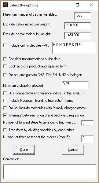
Explanation of this window:
1. Maximum number of causal variables: The program will calculate this based on the size and complexity of your database, up the maximum allowed (see previous paragraph). You can adjust this number here and in the Options menu.
2. Exclude by molecular weight (boxes 2 and 3): You can limit the analysis to only consider molecules between a minimum and maximum molecular weight.
3. Include only molecules with: - Check this box if you want to only want to analyze molecules containing specific atom types. You can modify which atoms you look for by adding or subtracting atomic symbols from the comma separated list.
4. Consider transformations of the data:
If checked, the program will try to determine the best transform for the data (i.e transform the experimental response parameter.) It will do this using only for the models of the count for each type of atom as independent variables (i.e. number of carbons, number of hydrogens etc.). The transforms of response used by MMP are a combination of: (a) multiply or divide by molecular weight and/or molecular volume with raw data, and (b) log10, square, square root or logistic and the inverse of these five transforms. A total of 70 different combinations of these factors will be analyzed. The program will choose one, then proceed with the rest of the analysis. If you do not choose to consider the transformations, the program will still see if the data is better fit by dividing all the atom counts (e.g. number of carbons, number of oxygens, etc.) by molecular weight (it will not do this if you select transformations, as multiplying the response by molecular weight is similar to dividing the independent variables by molecular weight.)
5. Look at cross product and squared terms. After the model completes the stepwise regression of all the independent variables, it will look the squares and cross products of all the terms in the model to see if they improve it further.
6. Do not amalgamate CH3, OH, SH, NH2, NO2 or halogen.
If checked, the method will use a simpler, faster set of fragments to analyze the data. You would complete the analysis sooner and perhaps have a more general model, but lose some of the structural information in the data.
MMP+ combines terminal groups, like H, OH, =O, =S, F, Cl, Br, I, NH2, #N, NO2 and CH3 with the atoms they are attached to in the default model. It also looks for concentrations of heteroatoms with structures: O[or N]C(=O) [or =S]N [orO]. If you check this box the program will only attach H, =O and =S.
If you check the box the molecule CH3CH2C(=O)NHCH2CH3 would generate the following pairs for analysis:
Number of C(H)(H)-C(H)(H)(H) pairs = 2; Number of C(=O)-C(H)(H) pairs = 1; Number of C(=O)-N(H) pairs = 1; Number of C(H)(H)-N(H) pairs = 1
If you left the box unchecked it would generate:
Number of C(H)(H)(CH3)-N(H) pairs = 1; Number of C(=O)-N(H) pairs = 1; Number of C(=O)-C(H)(H)(CH3) pairs = 1
In a database containing all kinds of molecules containing over 4000 values for log Kow, checking this box generated 400-500 unique combinations of pairs, while leaving the box uncheck generated over 1300 sub-structural features. Leaving the box unchecked gives a model containing more chemical information, with the danger that the model will be less general.
7. Minimum probability allowed. I have set the default at 0.05, the typical value used by statisticians. This appears to work even with data acquired from multiple sources from the internet. Setting this value correctly is a function of the accuracy of your data, and setting it high or low will effect where the analysis stops (how many independent variables are included in the model.) For highly accurate data this value should be set very low (molecular weight, for instance, could be set at p <=0.0001). For sharing in the literature, you may find resistance from reviewers or regulators with p > 0.05. [p = probability that an independent variable's correlation is due to chance. 0.05 means 5% probability.]
8. Use connectivity and valence indices in the analysis. This will cause the method to consider connectivity and valence indices 1 through 4 and the kappa shape index 2 in the analysis. If will not, though, force them into the model as an included variable. This feature is useful if you think the model should contain both whole molecule properties and sub-structural fragments in the model.
9. Include Hydrogen Bonding Interaction terms. The program will consider some additional variables if you check this box. It will look to see if each molecule contains more than one of the following features and will create a cross product of the number of each pair in every molecule. The H bonding groups it looks for are NH, NH2, OH, =O, COOH, SH, S(=O) and P(=O). In our example of CH3CH2C(=O)NHCH2CH3 this would create one additional term: NH x C=O. It would also create this term for the molecule O=CHCH2CH2NHCH3 (not just for amide.)
10. "Do not include molecules with formally charged atoms." Checking this box will eliminate molecules with formally charged atoms, for instance, Na+, Cl- from the analysis. It will eliminate most salts, for instance, from the analysis of the chemelectrica.mdb and mydata.mdb data sets.
11. Alternate between forward and backward regression. When this is checked the program will for do forward regression for a number of steps. Next it will add all the substructural features that had p<0.05 (or the significance selected in step 7 aobove) to the model and do a backwards regression. It will continue until no variable with p<0.05 or which increases r square by more than 0.0001 can be found and then do a final backwards regression. The program will do about 10 forward steps the first time, but thereafter will do the number of forward steps you specify in the line after the check box (default = 3 steps.) For large data sets, we recommend you keep this box checked, because it greatly speeds the analysis (answer in hours or days instead of weeks.)
If you do not check this box, then the model will do a forward regression all the way to the end and do a backwards regression only after no more significant variables can be added. Leaving this box unchecked can lead to a very long analysis with large, complex data sets (lasting weeks.)
12. Transform by dividing the variables by each other. Checking this box will cause the program to consider dividing every significant independent variable by each other. In conjunction with repeating the process (item 13 below) very complicated non-linear models are possible. It adds one to the denominator to avoid division by zero. A consequence of this is that it will also evaluate the x/(x+1) transform (dividing a variable by itself plus one which describes a curve converging on one.) Checking this option will greatly increase the time of analysis and may make the model less general (while better predicting that data in the database.) With repeated iterations (next paragraph) it can be used to model very complicated internal molecular interactions.
13. Number of times to repeat the process (max 5): If you check cross products and division, you will usually be able to get a better model by repeating the process by going back to the step of doing a combination of forward and backward regression, then repeating the combinations and divisions steps. The process looks like this:
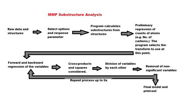
Usually two iterations are sufficient (keep the default 2), but sometime three will do it. Iterating the process will greatly lengthen the time of the analysis. Variables can become very complicated as cross product terms and division terms can be further multiplied and divided by each other.
14. Comments. If you would like to append a line of comments to the output file (author, references, explanation), place it here. For texts longer than a sentence or so, create a separate document.
After hitting the "Done" button, a new window appears from which you will select one response parameter (usually experimental data you wish to analyze.) Select a parameter and hit "Done."
Next a window will appear asking if you wish to force some variables from your database into the analysis. This allows you to combine the molecular properties calculated by MMP with sub-structural features of your dataset.
Next you will see all the molecules in the database flash by as the program determines the sub-structural features of the molecules. The program is not looking for specific features, but creates the sub-structural variables from scratch, depending on what combinations of atoms are contained in all the molecules in the database. After completing this, the log window appears and tells you how many molecules and variables will be included in the analysis. The program next looks for fields created that have the same exact values as other fields and for fields which have all the same values and eliminate these variables from the dataset. The program will display the names of the eliminated fields in the log window. The program proceeds with forward and backwards stepwise regression, adding parameters to the model until (a) no variables can be added that do not meet your significance level and the model r square does not improve by at least 0.0001 or (b) you hit the Cancel button. After completion the model will do a final backwards Stepwise regression to remove any variables that did not meet the level of significance that you specified, one step at a time starting with the least significant variable. If you selected cross products and squared terms, it will then look at all the combinations of the variables already in the model.
The program will ask you to save the dataset created by the program to a tab delimited text file. This will save the molecule names, the response (dependent variable), the predicted values, the molecular formula, the molecular weight, the connection table link and all the independent variable values. You can open up this database later in MMP or in Excel or any other program that opens tab delimited text files. Note this data will not be particularly secure. The program will also separately save all the information in the log window to a file called mmp.txt and open it with Notepad. If you want to save this log file save the file in Notepad and give it a different name.
After saving the data the program will display the model itself, as well as charts of predicted versus response and predicted versus residual values. Residuals are response minus expected values. Clicking on the data points to the far left or right of the residuals chart will identify the outliers (poorly predicted molecules.) Often these outliers are inaccurate experimental results. The file containing the model itself is automatically stored in the mmp\models subdirectory. This file is parsed by the program and should not be changed, though you can change the name of the file. If you share this file with other people and they put it in their mmp\models directory, then they will be able to use the file to predict properties of molecules using MMP.
To predict the value of the property for a molecule not in the database or for one which does not have an experimental value do the following:
1. Draw the molecule.
2. In the Drawing window go to the Calculate menu and choose "User Defined Properties." A new window will appear with a list of user defined properties. Click on the one you want and hit Run.
NOTE: MMP+ comes with models for boiling point, specific gravity and log Kow already in the \models folder. These models are used by the program to calculate these properties, so over-writing or deleting these files will change the default method used by MMP for calculating these properties. If you are dissatisfied with the way MMP calculates these properties you can re-run the analysis by opening the chemelectrica\mydata.mdb database, adding or removing molecules, editing the literature data fields, and re-running the substructure analysis. Running the log Kow analysis took about a week on an Intel I5 processor.
COMMUNITY SHARING PAGE:
New models will be published periodically at www.norgwyn.com/models/Models.html. You can download them there free of charge or submit new models for everyone to use that will appear on this web page. From the web page, just download the model text file into your mmp\models subdirectory and they will be usable from the Calculate/User Defined Properties menu of MMP.
A brief explanation of what is in the file for the model:
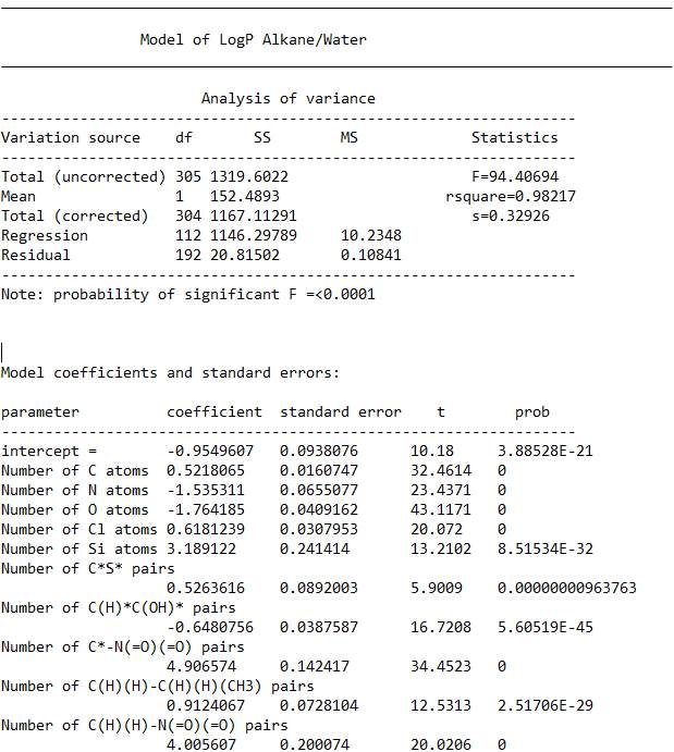
====================================================================
The Total (uncorrected) number of 305 is the number of molecules contained in the final model. (df stands for degrees of freedom)
The number 112 next to “Regression” is the number of variables. You usually want about 4x more molecules than variables, depending on the quality of the data.
The larger the F score, the better the model. The probability of the F statistic being significant is shown below the table.
R squared multiplied by one hundred is the percent of the variance explained by the model.
S is the model standard deviation. The 95% confidence level is twice this, plus or minus.
Below the analysis of variance table, you can see the first terms in the model itself. The format is, name of the variable, the coefficient that is multiplied by the number of time the substructure appears in a molecule and the standard error, t score and probability that the term is significant (0 is a term so significant, the program could not determine the value.)
To predict the value of the property for a molecule not in the database or for one which does not have an experimental value do the following:
1. Draw the molecule.
2. In the Drawing window go to the Calculate menu and choose "User Defined Properties." A new window will appear with a list of user defined properties. Click on the one you want and hit Run.
NOTE: MMP+ comes with models for boiling point, specific gravity and log Kow already in the \models folder. These models are used by the program to calculate these properties, so over-writing or deleting these files will change the default method used by MMP for calculating these properties. If you are dissatisfied with the way MMP calculates these properties you can re-run the analysis by opening the chemelectrica\mydata.mdb database, adding or removing molecules, editing the literature data fields, and re-running the substructure analysis. Running the log Kow analysis took about a week on an Intel I5 processor.
3.
ATOM BASED ANALYSIS
NOTE: This routine uses lots of RAM and lots of CPU time and can take a long time to complete if you have a database of over 1000 molecules in it.
To access this feature: Open a database. Go to the Analyze menu. Choose the second item, "Atom Based Analysis." This feature differs from the Substructure Analysis in two ways. It (1) starts the substructure from specific atoms using qualifications such a charge, lipophlicity or location, while ignoring the other atoms AND (2) will create substructures of many connected atoms, going more deeply into the structures. For instance, you could restrict an analysis of pKa to structure starting from the most positively charged hydrogen atoms or you could restrict analysis of a polymer database to starting with the two end atoms. You could model a receptor by starting the substructures with up to 10 of the most negatively charged atoms and include distances between the atoms from left to right along the x axis.
Like the substructure analysis, this method will create substructures from the molecules in your database which will be used as independent variables in the analysis. This routine uses least squares multiple regression to find the substructural features that are significantly correlated with the property being modeled and places the model in your \atom_based subdirectory. After completing the analysis, this property can be predicted for any molecules you draw by selecting "user defined properties" from the Calculate menu of the Drawing window.
What can be analyzed: This method does not care what atom types you have in your database. It creates the substructures from the molecules themselves, not from a look-up table. You should be able to analyze any set of molecules as long as you have input the structures correctly. Molecules should be drawn in a consistent manner (e.g. if you draw nitro as N(=O)=O one time and N+(=O)O- the next it will not recognize them as the same substructure. Salts and ionic molecules are also types of molecules that can be drawn in many different ways.)
CAVEAT EMPTOR: On large databases this method will take days to complete the task. On a database of 72 structurally related molecules this method takes a few minutes to complete its task on a slow XP computer. On a database of 800 molecules containing mostly solvents and surfactants, this method took 2 hours to complete its task on a slow XP computer. On a database containing over 4000 molecules with over 1300 unique sub-structural features on an Intel I5, Windows 10 computer the program took about a week to converge. Fortunately, the computer was still usable as the task ran in the background. However, the database being used was tied up for the duration of the analysis. The length of the task is a function of your computing speed. The size of the database that can be used is limited by RAM. If you expect to routinely use this program feature on large databases, we recommend you have a computer dedicated to the task.
Details of the Method:
The number of variables that will be generated is a function of the size and complexity of the structures in the database. The default setting for maximum number of sub-structural variables is 1800. If you get an "out of memory" error go to the Options menu of the Database window and decrease the number of variables allowed in the analysis. If using the mydata.mdb or chemelectrica.mdb database you will need to set this to about 2500 because the program will find over 2000 substructures with the atom depth set to 4.
After selecting "Atom Based Analysis" from the Analyze menu of the Database window the following Window will appear:
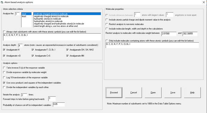
Explanation of this window follows:
Atom Selection Criteria:
1. In the upper left you choose what types of atoms to
start the substructure generation and how many.
You can choose to analyze 1-10 atoms per molecule. You can choose select starting atoms by
charge, lipophilicity or the two atoms at the two ends of the molecule oriented
along the x axis.
2. You can restrict the starting atoms by atomic symbols
in a comma separated list. If you want
to start the substructures with hydrogen, for instance, you would check the box
“Always start substituents with atoms with these atomic symbols” and then
change the text below this check box to read “H”.
3. Analysis depth determines how deeply the program with
delve into the molecule from the starting point. For instance, if you have opted to look at
the one most positively charged hydrogen atom as your starting point and have
an analysis depth of 4, for n-hexanoic acid you would generate the following
substructures:
With Amalgamate H, =O and OH checked: C(=O)(OH), C(=O)(OH)C(H)(H), C(=O)(OH)C(H)(H)C(H)(H), and C(=O)(OH)C(H)(H)C(H)(H)C(H)(H).
With Amalgamate H, =O and OH unchecked: H, OH, HOC, and
HOC(=O)C(H)(H).
Analysis Options:
1. Check boxes for transforming the dependent variable
(the parameter being modeled.) can be checked as desired. Your options are, 1/x, x/molecular weight and
log10(x) or any combination of these three.
2. Cross products and squares of the independent
variables (e.g. the substructures) will be considered in the analysis (i.e.
y1*y2, y1*y1
etc.). Only the variables found to be
likely to be significant will be used.
3. Divide the
independent variables by each other.
Checking this box will cause the program to consider dividing every
likely-significant independent variable by each other. In conjunction with repeating the process
very complicated non-linear models are possible. It adds one to the denominator to avoid
division by zero. A consequence of this
is that it will also evaluate the x/(x+1) transform (dividing a variable
by itself plus one which describes a curve converging on one.) Checking this
option will greatly increase the time of analysis and may make the model less
general (while better predicting that data in the database.) With repeated iterations (next paragraph) it
can be used to model very complicated internal molecular interactions. This feature is the one most likely to
generate spurious correlations (due to the number of possible variables being
much greater than the number of observations.)
4. Iterate the process.
If this number is greater than one, the program will, after determining
cross products and division go back to the beginning of the analysis and repeat
the process to see if there were any significant variables missed before doing
the cross-products, squares and divisions.
5. Forward step to take before going backwards. The program will do a standard forward
stepwise regression for the selected number of steps (more the first time
through). Then it will accelerate the
analysis be adding all the significant independent variables it found and do a
backwards stepwise regression. Next it
will do the forward regression and repeat this process until there are no more
variables with 3x of the selected probability cut-off. At the end of the analysis (including the
cross products and divisions)
all the variables still having a probability above the cut-off
(usually p=0.05) will be removed by a final backwards regression.
6. Probability of chance cut-off for independent
variables: The default is set at 0.05, the typical value used by statisticians.
This appears to work even with data acquired from multiple sources from the
internet. Setting this value correctly is a function of the accuracy of your
data, and setting it high or low will affect where the analysis stops (how many
independent variables are included in the model.) For highly accurate data this
value should be set very low (molecular weight, for instance, could be set at p
<=0.0001). For sharing in the literature, you may find resistance from
reviewers or regulators with p > 0.05. [p = probability that an independent variable's
correlation is due to chance. 0.05 means 5% probability.]
Molecular Properties:
1. Include distances between [variable] atoms [variable)
angstroms apart: This check box only is
enabled when you analyze more than one starting atom. It will create independent variables for the
distances between the starting atom points.
2. A) Include partial charge and dipole moment in the
analysis: This check box causes the
partial charge of the starting atoms to be included as an independent variable
as well as the molecular dipole moment as calculated by CNDO. It is available if you used partial charge as
the criteria for selecting the starting atoms.
B) Include atomic lipophilicity values in the
analysis. This check box causes the
lipophilicity score of the starting atoms to be included as an independent
variable. It is available if you use
hydrophilicity or hydrophobicity as the determinant for the starting atoms.
3. Restrict molecules to non-ionic molecules: Excludes
all molecules with formal charges.
4. Include molecular length width and depth in the
calculations: Includes the length (along
x axis), width (y axis) and depth (z axis) of the molecules as independent
variables in the analysis.
5. Restrict molecular weight to molecules between [lower
bound] and [higher bound]: You can limit the analysis to only consider
molecules between a minimum and maximum molecular weight. The default is the full range of molecular
weight present in the database.
Use Molecular Geometry in the
Calculations:
These options will only be visible if more than one atom is used as a starting point and the Include distances between atoms check box under molecular properties is checked.
1. Sort atoms from left to right along the x axis. The starting atoms will be sorted by their
position along the x axis. If not
checked, the atoms will be sorted by how large the charge or hydrophobicity
score is. 2.
2. Orient molecules with maximum length along the x axis
and maximum width along the y axis: Before doing other calculations, each
molecular will be rotated so that the largest possible length and largest width
perpendicular to that length is made.
3. Rotate the molecule 180 degrees along Y is the X
component of dipole moment is negative and 180 degrees around the X axis if the
Y component of dipole moment is negative.
It does this AFTER rotating the molecular for maximum x and maximum y if
check box 2 above is checked. The check
box is only enabled if you select charge as the criteria for choosing the
starting atoms.
4. Rotate the molecule 180 degrees so that the most
lipophilic half is on the right side. It
does this AFTER rotating the molecular for maximum x and maximum y if check box
2 above is checked. The check box is
only enabled if you select charge as the criteria for choosing the starting
atoms.
5. Save changes in the atom’s orientation (i.e. if you
selected any of 2-4 above) to the database.
This may save time if you repeat the analysis. Note that if your molecular structures are
stored as separate files, the change in geometry will be saved to the files,
and made permanent. If, on the other
hand, you save the geometries within the database, then you must later save the
database to make the changes permanent.
After hitting the "Proceed" button, a new window appears from which you will select one response parameter (usually experimental data you wish to analyze.) Select a parameter and hit "Done."
Next a window will appear asking if you wish to force some variables from your database into the analysis. This allows you to combine the molecular properties calculated by MMP with sub-structural features of your dataset.
Next you will see all the molecules in the database flash by as the program determines the sub-structural features of the molecules. The program is not looking for specific features, but creates the sub-structural variables from scratch, depending on what combinations of atoms are contained in all the molecules in the database. After completing this, the log window appears and tells you how many molecules and variables will be included in the analysis. The program next looks for fields created that have the same exact values as other fields and for fields which have all the same values and eliminate these variables from the dataset. The program will display the names of the eliminated fields in the log window. The program proceeds with forward and backwards stepwise regression, adding parameters to the model until (a) no variables can be added that do not meet your significance level and the model r square does not improve by at least 0.0001 or (b) you hit the Cancel button. Cancelling goes to the next step in the analysis, not necessarily the end. After completion the model will do a final backwards Stepwise regression to remove any variables that did not meet the level of significance that you specified, one step at a time starting with the least significant variable. If you selected cross products and squared terms, it will then look at all the combinations of the variables already in the model.
The program will ask you to save the dataset created by the program to a tab delimited text file. This will save the molecule names, the response (dependent variable), the predicted values, the molecular formula, the molecular weight, the connection table link and all the independent variable values. You can open up this database later in MMP or in Excel or any other program that opens tab delimited text files. Note this data will not be particularly secure. The program will also separately save all the information in the log window to a file called mmp.txt and open it with Notepad. If you want to save this log file save the file in Notepad and give it a different name.
After saving the data the program will display the model itself, as well as charts of predicted versus response and predicted versus residual values. Residuals are response minus expected values. Clicking on the data points to the far left or right of the residuals chart will identify the outliers (poorly predicted molecules.) Often these outliers are inaccurate experimental results. The file containing the model itself is automatically stored in the mmp\models subdirectory. This file is parsed by the program and should not be changed, though you can change the name of the file. If you share this file with other people and they put it in their mmp\models directory, then they will be able to use the file to predict properties of molecules using MMP.
To predict the value of the property for a molecule not in the database or for one which does not have an experimental value do the following:
1. Draw the molecule.
2. In the Drawing window go to the Calculate menu and choose "User Defined Properties." A new window will appear with a list of user defined properties. Click on the Atom Based button. Click on the property you want and hit Run.
COMMUNITY SHARING PAGE:
New models will be published periodically at www.norgwyn.com/models/Models.html. You can download them there free of charge or submit new models for everyone to use that will appear on this web page. From the web page, just download the model text file into your mmp\models subdirectory and they will be usable from the Calculate/User Defined Properties menu of MMP.
This routine will perform multiple regression analysis using least square minimization. The user selects the following:
1. The result parameter (dependent variable)
2. Up to twenty-four causal parameters (independent variables). When the final causal parameter is selected, choose 'none' from the parameter list or the DONE button at the bottom to begin the multiple regression analysis.
The program will come back with the following information:
1. A correlation matrix between the parameters in the model.
2. The eigenvectors and eigenvalues used.
3. Analysis of variance table:
df are "degrees of freedom"
SS are "sums of squares"
MS are "mean squares"
4. r square, F, model standard deviation, model probability
r square is the proportion (of 1) of the variance explained by the model (0.99 = 99% of variance explained).
F is the proportion explained divided by 1-proportion explained.
s is the model standard deviation, a measure of how uncertain the predicted values are.
The probability of significant F is the probability that the model is due to chance alone (1 = chance, 0.05 means a 95% confidence that the model is not due to chance, but is due to the causal variables in the model). The lower this number the better the model.
5. Intercept and parameter coefficients, standard errors, F values and the probability that a parameter is not significant.
The parameter coefficient is the actual value that the causal parameters are multiplied by in the predictive equation to obtain the predicted values.
The standard error column is a measure of the error in the coefficient term.
The students t value in this table is the proportion of variance explained divided by the proportion unexplained for the one variable model derived from the causal parameter.
The prob column is the likelihood that the parameter t value is due to chance alone.
6. A table of observed, predicted and residual values will be printed. All of the above will appear in a Windows Notepad screen. You can edit this file to suit yourself and save it under a new name or print it out.
observed values are the original experimental data points.
predicted values are those computed from the regression model.
residuals are the difference between the observed and predicted values.
7. If desired, the a regression plot of observed versus predicted and predicted versus residual values is plotted. The plot of observed versus predicted values should be highly correlated with a uniform variance. Plots whose points make a triangular, diamond or bow shape are missing significant causal variables or are needing a transformation in either the result or causal variable(s). The plot of the residuals should appear to be a random scatter plot (indicating uniform variance). If you want to identify outliers click the left mouse button on a point in these two plots. Clicking the right mouse button on a point will color it, highlighting it for presentations. To print out this plot select "Print Graphics Window" and "To a Printer" from the File menu, or select Automatic print before starting the plot.
8. For two variable models, a contour plot can be plotted with the first causal variable used as the x axis, the second causal variable used as the y axis, and the contours are colored by values of the result. To print out the contour plot select "Print Graphics Window" and "To a Printer" from the File menu after the contour plot is drawn or check the Automatic Print item on the Options menu.
9. You select whether you want to do a PRESS (predictive residual sum of squares) cross-validation of the regression analysis. PRESS leaves out each observation and calculates the regression equation without it. It then determines the square of the residual value of the observation result minus the predicted value from the model calculated without it. PRESS adds these square terms together to obtain a total PRESS result. Observations which contribute large amounts to PRESS are probably outliers or influential observations. They should be examined. If the PRESS value is smaller than the sum of squares of the response (SSY) then the regression model is not just due to chance. Good models have the ratio PRESS/SSY <0.4. Excellent, highly predictive models have ratios less than 0.1. If you obtained the model first using the "Regress All Variables" model finder, then using the PRESS procedure is recommended to help avoid obtaining spurious correlations.
10. The compounds in the data base with the highest predicted value of result are listed at the end of the Notepad file containing the PRESS results (Regress.txt).
The maximum number of causal variables in the model is 25. If you want to include square and cross terms then you must make them with the "Transform a parameter" option below.
Partial least squares analysis
Partial least squares analysis is an alternative to ordinary multiple regression analysis that has advantages if:
a) your causal (y) variables are intercorrelated
b) you have a high ratio of causal
(y) variables to observations (multiple regression works best if there are no
less than 4 observations per y variable).
Multiple regression may still be used in the above cases, but answered may be “biased”. The PLS technique, popularized in the late 1980s, attempts to address this problem. A more detailed description of PLS is given in the part of this manual describing QSAR and QSPR studies.
MOLECULAR MODELING PRO
╖ Asks the user to choose the x (result) variables (yes there can be more than one), choose the y (causal) variables and choose between the following options:
a) Automatic printing -- this prints some results as the program executes, but in most cases will not be useful. In all cases, the results will be printed to a NotePad screen at the end. Printing, editing, cutting and pasting can be done from the NotePad window.
b) Include a cross-validation routine to choose the number of PLS components. This is recommended. Even if you do not want to use the recommended number of components, it is wise to look at the cross-validation results. The PLS routine uses a technique known as partial PRESS for cross-validation. It usually divides the data into four groups. It leaves out one group, does the PLS analysis, then sees how well the analysis predicts the group left out. The results for the total partial PRESS result are divided by the sum of squares of the Ys (SSY), to see how well the model is doing. A low PRESS/SSY is desirable. If this number is >0.5 then the model is a poor predictor, explaining less than 50% of the variance in Y.
c) Subtract the column means. This is recommended. If left out the final model will have no intercept.
d) Show all the vectors in the NotePad print-out. If you want to see the t, u, p, r and q vectors, than check the box.
e) Number of principal components. If you do not choose to do cross-validation, then this is the number of components that will be used. If you use cross-validation, then this is the maximum number of components that will be used.
╖ The program will execute as follows:
a) The cross-validation will be run. The user chooses if he wants to use the recommended number of components. Otherwise the maximum number of components will be used.
b) The PLS analysis will be done.
c) The user can then plot some of the results of the analysis in 2-D. Vectors that can be plotted include raw ys, raw xs, predicted y, residuals, and the t and u vectors.
d) A NotePad window will appear with the results of the analysis
╖ In the NotePad window appear the following statistics:
1. The results of the cross-validation routines. Good models have the PRESS/sum of squares of Y <0.5.
2. The column means and variances for the raw x and raw y data.
3. The principal component loadings
4. The results for all the PLS vectors and matrices if requested. Note that these results are printed in files anyway (e.g. PLS_T.txt)
5. The model in standard multiple regression form:
Y = Intercept + A(Y1) + B(Y2) + C(Y3) +
etc.
6. The raw Y, predicted Y and residual for all observations. This includes predicted values for compounds where all Xs (causal variables) are known, but the Y (response) is not known.
Principal components regression
Principal components regression first calculates the eigenvalues and eigenvectors formed by you independent variables. Then, it uses the eigenvectors as the independent variables in multiple regression analysis. The idea here is that the eigenvectors are the real underlying causes of variation in the data, especially when they are composed of many of the original independent variables. The main problem with this technique, is that it is hard to convert the principal components (eigenvectors) back into reality. For instance we know what surface tension or Log P is. But how do we interpret a principal component that is 10% surface tension, 40% Log P, 15% molecular volume and 35% molecular length? For this reason, multiple regression analysis using the original independent variables is usually more useful for applied research. However, you can use this routine to predict results for any compound for which you have a all the causal variables (Xs), and in some circumstances this may be useful.
A description of the statistics printed to NotePad by this routine can be found in the description of multiple regression.
Don't want to miss the best model? Not afraid of misinterpreting spurious correlations? Then this is the method for you. This method regresses the selected response variable with all the other parameters. Simply select the response variable, the excluded parameters, 0-5 included parameters, and tell it the cut-off (1-4 unincluded variables allowed). If you have a large data base (e.g. >25 fields) and a slow computer then having 3 as the cut-off can take 15-60 minutes and 2 hour or more job. Look models over carefully with the multiple regression routine above (including plotting out data, and use of the PRESS cross-validation method), and make sure that they make sense, before exclaiming "Eureka". Selecting Automatic print from the Regressions options panel that appears at the start of the "Regress All" routine will cause all data to be printed after completion of the analysis.
Options:
1. Include transformations: One variable models with the following transformations of both x and y will be considered: reciprocal (1/x, 1/y), log(), logistic(), 1/log(), x and y squared, and square root of x and y. The best ten variable transformed y terms will be carried over into the 2-4 variable models. It also will look at the best x transform (as well as untransformed x) in the 2-4 variable models.
2. Non-linear combinations: the independent variables will be combined by looking at all possible combinations of them multiplied together, divided by one another and subtracted from one another. The best 10 terms will be carried over into the 2-4 variable models.
The routine will also look at models with the following patterns: x = y + y2 (reported with 2 variable models), x = y1 + y2 +y1*y2 and x = y + y2 + y3 (reported with 3 variable models).
Note: in order to speed
execution, this routine places the entire database in
Note: Natural logs are used (not base 10). For the logarhythmic and logistic transformations if there are values of zero or less, a number equal to the minimum values plus the range divided by 100 is added to all the numbers. The logistic transform is ln(y/(1-y)) where y has been scaled to numbers from 0.000001 to 0.999999 by dividing all the numbers by the range.
Strategy hint: With large databases, 4 variable models with transformations can take hours to calculate. Instead choose to only do the 1 and 2 variable models, examine the results and use the best 2 variable model parameters as included parameters in a second iteration through the routine.
To access this feature: Open a database. Go to the Analyze menu. Choose the first item, "Stepwise regression."
What this analysis will do: After you choose the property to model, this method will attempt to correlate it with a combination of all the other properties in your database. It will then use Stepwise multiple regression to find the properties that are significantly correlated with the response you choose and places the model in your \stepwise subdirectory. You can then predict the property of any molecule you draw from the Drawing window by selecting "user defined properties" from the Calculate window.
Except for using the MMP calculated molecular properties instead of substructure fragments, this method is almost identical to the "Substructure Analysis" detailed in the previous section. An additional window will appear that allows you to exclude properties from the analysis. The Stepwise method will usually be faster than the Substructure Analysis because there are fewer potential independent variables to analyze.
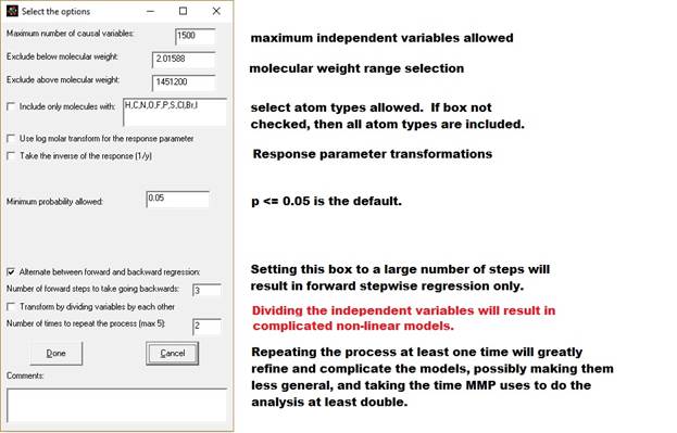
1. Maximum number of causal variables: The program will calculate this based on the size and complexity of your database, up the maximum allowed (see previous paragraph). You can adjust this number here and in the Options menu.
2. Exclude by molecular weight (boxes 2 and 3): You can limit the analysis to only consider molecules between a minimum and maximum molecular weight.
3. Include only molecules with: - Check this box if you want to only want to analyze molecules containing specific atom types. You can modify which atoms you look for by adding or subtracting atomic symbols from the comma separated list.
4. Use log molar transform: After checking this box, your dependent variable (response variable) will be transformed before analysis, i.e., y will become log10(y/molecular weight). Note that the data will be transformed back to the original transform when determining properties of new molecules with unknown property values.
5. Take the inverse of the response. After checking this box your dependent variable will be transformed before analysis (i.e. y will become 1/y).
6. Minimum probability allowed. I have set the default at 0.05, the typical value used by statisticians. This appears to work even with data acquired from multiple sources from the internet. Setting this value correctly is a function of the accuracy of your data, and setting it high or low will effect where the analysis stops (how many independent variables are included in the model.) For highly accurate data this value should be set very low (molecular weight, for instance, could be set at p <=0.0001). For sharing in the literature, you may find resistance from reviewers or regulators with p > 0.05. [p = probability that an independent variable's correlation is due to chance. 0.05 means 5% probability.]
7. Alternate between forward and backward regression. When this is checked the program will for do forward regression for a number of steps. Next it will add all the substructural features that had p<0.05 (or the significance selected in step 7 aobove) to the model and do a backwards regression. It will continue until no variable with p<0.05 or which increases r square by more than 0.0001 can be found and then do a final backwards regression. The program will do about 10 forward steps the first time, but thereafter will do the number of forward steps you specify in the line after the check box (default = 3 steps.) For large data sets, we recommend you keep this box checked, because it greatly speeds the analysis (answer in hours or days instead of weeks.)
If you do not check this box, then the model will do a forward regression all the way to the end and do a backwards regression only after no more significant variables can be added. Leaving this box unchecked can lead to a very long analysis with large, complex data sets (lasting weeks.)
8. Transform by dividing the variables by each other. Checking this box will cause the program to consider dividing every significant independent variable by each other. In conjunction with repeating the process (item 13 below) very complicated non-linear models are possible. It adds one to the denominator to avoid division by zero. A consequence of this is that it will also evaluate the x/(x+1) transform (dividing a variable by itself plus one which describes a curve converging on one.) Checking this option will greatly increase the time of analysis and may make the model less general (while better predicting that data in the database.) With repeated iterations (next paragraph) it can be used to model very complicated internal molecular interactions.
9. Number of times to repeat the process (max 5): If you check cross products and division, you will usually be able to get a better model by repeating the process by going back to the step of doing a combination of forward and backward regression, then repeating the combinations and divisions steps.
Usually two iterations are sufficient (keep the default 2), but sometime three will do it. Iterating the process will greatly lengthen the time of the analysis. Variables can become very complicated as cross product terms and division terms can be further multiplied and divided by each other.
10. Comments. If you would like to append a line of comments to the output file (author, references, explanation), place it here. For texts longer than a sentence or so, create a separate document.
After hitting the "Done" button, a new window appears from which you will select one response parameter (usually experimental data you wish to analyze.) Select a parameter and hit "Done."
Next a window will appear asking if you wish to force some variables from your database into the analysis. This allows you to combine the molecular properties calculated by MMP with sub-structural features of your dataset.
The list of properties will appear again and this time you select properties to exclude from the analysis (otherwise the program will look at every numeric field in the database.)
The program looks for fields created that have the same exact values as other fields and for fields which have all the same values and eliminate these variables from the dataset. The program will display the names of the eliminated fields in the log window. The program proceeds with forward and backwards stepwise regression, adding parameters to the model until (a) no variables can be added that do not meet your significance level and the model r square does not improve by at least 0.0001 or (b) you hit the Cancel button. After completion the model will do a final backwards Stepwise regression to remove any variables that did not meet the level of significance that you specified, one step at a time starting with the least significant variable.
The program will ask you to save the dataset created by the program to a tab delimited text file. This will save the molecule names, the response (dependent variable), the predicted values, the molecular formula, the molecular weight, the connection table link and all the independent variable values. You can open up this database later in MMP or in Excel or any other program that opens tab delimited text files. Note this data will not be particularly secure. The program will also separately save all the information in the log window to a file called mmp.txt and open it with Notepad. If you want to save this log file save the file in Notepad and give it a different name.
After saving the data the program will display the model itself, as well as charts of predicted versus response and predicted versus residual values. Residuals are response minus expected values. Clicking on the data points to the far left or right of the residuals chart will identify the outliers (poorly predicted molecules.) Often these outliers are inaccurate experimental results. The file containing the model itself is automatically stored in the mmp\stepwise subdirectory. This file is parsed by the program and should not be changed, though you can change the name of the file. If you share this file with other people and they put it in their mmp\stepwise directory, then they will be able to use the file to predict properties of molecules using MMP.
After saving the data the program will display the model itself, as well as charts of predicted versus response and predicted versus residual values. Residuals are response minus expected values. Clicking on the data points to the far left or right of the residuals chart will identify the outliers (poorly predicted molecules.) Often these outliers are inaccurate experimental results. The file containing the model itself is automatically stored in the mmp\stepwise subdirectory. This file is parsed by the program and should not be changed, though you can change the name of the file. If you share this file with other people and they put it in their mmp\stepwise directory, then they will be able to use the file to predict properties of molecules using MMP.
After the analysis is done, to predict the value of the property for a molecule not in the database or for one which does not have an experimental value do the following:
1. Draw the molecule.
2. In the Drawing window go to the Calculate menu and choose "User Defined Properties." A new window will appear with a list of user defined properties. Click on "Go to Stepwise Directory" (unless already clicked.) Click on the property you want and hit Run.
This menu item, when selected, prints out the parameter names, number of non-missing values, mean, minimum, maximum, sum, and standard deviation. Results appear in a Notepad window which can be saved, printed or cut and pasted to another application.
Correlation matrix (all variables)
Prints out a list of the correlations of all parameters in the database with each other and lists the Pearson's r value.
Calculates the
Raw data
========
Result for sarcoma E-235555 Control
-----------------------------------------------------------------------
Progress Free Survival (6 mos) 17 6
Progressive Disease 61 72
===========================================================================
Expected frequencies
====================
Category E-235555 Control
-----------------------------------------------------------------------
Progress Free Survival (6 mos) 11.5 11.5
Progressive Disease 66.5 66.5
===========================================================================
Chi Square: 6.170644
Probability: 0.005-0.01 directional, 0.01-0.02 non-directional
degrees of freedom for determination of probability: 1
Total number of Observations: 156
You can save and open data from
the file menu. Raw data can be changed
with the backspace key, the alphanumeric keys and the add row and delete rows
button. You can navigate through the raw
data grid using the enter key. When the
raw data is correctly entered hit the Compute button to obtain the
Transform a parameter
The user selects the parameter to transform, the transformation to be used and the field position (which text box will be used on the file card utility). The transformations available are:
1. untransformed: (copy the field)
2. square: (x*x)
3. square root: (sqr(x))
4. inverse: (1/x)
5. log: (ln(x))
6. log molar: (molecular weight of x/log10(x))
7. logistic: (ln(x/(maximum x-x)))
8. binomial: (sqr(arc sine x))
9. negative binomial: sqr(1-X)-((1-x)^1.5)/3
10. multiply x by a second parameter
11. add x to a second parameter
12. subtract a second parameter from x
13. divide x by a second parameter
14. multiply x by a constant
15. add a constant to x
16. subtract a constant from x (if you want to subtract x from a constant you must add the negative value of x to the constant.
17. divide x by a constant (if you want to divide a constant by x you must multiply the constant by 1/x).
18. cosine(x)
19. sine(x)
20. tangent(x)
21. arc tangent(x)
|
These menu items compare the similarity of the displayed molecule in the Drawing window with all the molecules in a database. Differences in physical and chemical properties are divided by the range in the property in an attempt to scale the properties relative to each other. The total difference is the simple sum over the scaled differences in the properties. Note that if the property fields do not exist in the database then the similarity calculations cannot be made. - Similarity using all fields: All calculated fields are used in the calculation. Tip: note that if you do this on the substructure keys file (yourdatabaseName.ssf) the similarity results will closely resemble a structural similarity search. |
|
|
- Similarity using solubility parameters: The 3-D solubility parameters are used (dispersion, polarity and hydrogen bonding). This can be useful for looking for solvent replacement needs. |
|
|
- Similarity using bioavailability parameter: The properties used in the Lipinsky Rule of 5 determination are used (Moriguchi log P, molecular weight, number of hydrogen bond acceptors and donors, and polar surface area). Will find molecules, that in theory, are transported across biomembranes similar to the molecule drawn. |
|
-Similarity using substruture keys - The substructure keys database (.ssf), a standard csv file is used to estimate the similarity to the molecule drawn. In addition, connectivity and valence indices (Randic, Kier and Hall type indices) are used for additional comparisons. Substructural keys contain many common features of molecules such as number of aromatic carbon atoms, number of amide groups, number of nitro groups etc. All of the above routines under the Compare menu use the Jaccard/Tanimoto method of comparing the molecules: Sij = a/(a+b+c) where a is the data in common and b and c are the data unique to each molecule. This method is considered the most accurate means of identifying similar molecules (Chen et.al., J. Chem. Inf. Model. 46: 478-486 [2006]). The value presented to the user by MMP Plus is the mean S value for all the non-missing fields. If over 5% of the fields are missing, the value is not reported. |
The Options Menu
Create Back-up on Opening - when this is checked, MMP will create a back up of the database opened automatically. The file name will be like the file name opened, but with the file extension .bak.
View structures as mixtures or reactions: This menu item is only available to ACCESS data bases with a reaction_table (molecules stored as reactions during database creation). If checked, the molecules will display as reactions. If unchecked the molecules will display individually.
Include Hydrogens in Substructure Searches. This will do what it implies.
Set Maximum Number of Variables in Substructure Analysis and Stepwise
Regression. The default was set to 1001
to avoid out of memory errors on old computers.
If you have a large, structurally diverse dataset (>2000 molecules)
you may need to make this number larger.
For instance, a dataset containing about 4100 molecules of all types
required this number to be set to 1400 which ran on a computer with an I5
processor and 6 MB of
Handling Fields
Adding new fields from the Edit menu (Fields/Add fields) is simple enough. A field creation window appears and you type in the names of the field and select the type of data from the list (text, memo, single precision number, integer etc.). Hit the OK button on the bottom left after typing in the field name and type. You can then type in additional field names with data types (add as many new fields as you like). Hit the 'Done' button at the lower right when finished and the fields will be created. If the name of the field matches one of the field names calculated by MMP, the program will calculate it. A list of names the MMP understands is in the file fldnames.txt. In the left hand pane of the Field Addition window you can bring up this list by hitting the button entitled Get Field from a list. You can select all of the common calculated fields by checking the box entitled "Check all commonly calculated fields." Remember to save the database or the new field names and any new data types into the field's records will not be saved!
Alternative method for adding new fields: Open the data base. Save it to the EXCEL option. This opens the data base in EXCEL. Type in a new field name in the first unused column. Type in any data that you want (you can do this in MMP too). Select the area in EXCEL that contains the field names and all the data. Copy it to the clipboard. In the MMP DATABASE window, Open the data base by Pasting tab-delimited text from the clipboard (the last item on the Open menu). If you are adding fields to an ACCESS reaction data base, click on the "Yes" button the program asks if you would like to keep the current reaction table. Otherwise this table will be deleted (ACCESS data bases created by MMP contain three tables "Data_Table, Pindex_Table and Reaction_Table). The new fields and data do not become permanent until you save the data.
Note that you can also use EXCEL to delete fields, change the field names and the order in which the columns are displayed.
There are many other ways to add fields to the database, but all involve going to another program to do it. For instance, you could copy the database to the clipboard (File/Save/Copy tab-delimited database to the clipboard menu items) and paste it into another program. Then proceed as above (the program has mainly been tested with EXCEL though). If you are using the ACCESS data base format, note that you cannot copy the reaction table, only the data table.
Need more help? You can e-mail Norgwyn Montgomery Software at info@norgwyn.com. Visit our web sites at http://www.norgwyn.com (developer) for information about our products. For suggestions about improving the product send e-mail to Dr. James Quinn, Chief Programmer of Norgwyn Montgomery Software Inc.