|
|
Molecular Modeling
Pro Plus Drawing Window Menus |
|
File | Edit | Format | Tools | Rotate | Calculate | Geometry | Display | Slides | Help |
|
|
MMP+ Main Help page | The Database Window
- menu item descriptions | The Image Processor |
|

Overview
The
File menu contains
routines for opening and saving structure files and for opening, saving and creating databases. It
also contains some printing routines. The Edit menu contains methods for copying and pasting graphics or connection tables to the clipboard and
allows the user to add text and bulleted lists to the graphical display. The Format menu has methods for controlling which molecular
properties provide the coloring schemes of atoms and molecules. The Tools menu is the entry point for the Reaction
editor, Huckel MO
calculations, CNDO, MOPAC, the html image generator and substructure searching. The Rotate menu is one entry point to molecular and bond
rotation routines (clicking on
the screen with the right mouse button is another). The Calculate menu is the entry point for calculating molecular
properties from structure, such as molecular dimensions, charge and dipole
moment, solubility, bioavailability, thermodynamics, and polymer specific
properties. The Geometry menu contains methods for conformational analysis, minimization and molecule-molecule docking. The Display menu allows the user to change how the molecule is
displayed and labeled and set z-plane
clipping. The Slides menu contains methods for creating a computer slide
show. The Help menu brings up the files you are looking at.
New
Clears all molecules and bitmaps from the screen.
Open
Selecting this menu item causing the standard
Microsoft Open dialog box to appear. At
the lower left of this dialog box is a list of connection table file
formats. A connection table is the file
where structural information about your molecule is stored. The supported file types are:
MACROMODEL file
Molfile
Reaction or mixture
Ring files (MACROMODEL format)
Brookhaven pdb files
MOPAC Input file
MOPAC Output file
Bitmaps and metafiles
Select the file format desired, the directory to
open it from and the molecule from the file list box. The molecule should open.
Description
of file formats:
MACROMODEL
files (*.dat)
This format originated with the MACROMODEL program
developed at
MDL Molfiles (*.mol)
This is a good choice for molecules with formal
charge or for molecules that you wish to share with other programs. MDL Molfiles are
the standard ASCII text connection table format recognized by most chemistry
software programs. The default version
used here is version 2000, which has a serious limitation (999 atom limit). If there are more than 999 atoms in the
molecule, MOLECULAR MODELING PRO
MOLECULAR
MODELING PRO
The individual molecules are stored as MACROMODEL
files, but there is an additional file containing information about the
reaction itself that ties the molecules together. This type of file is created by the Reaction
editor (Tools menu).
Ring files (*.rng)
These molecules are stored as MACROMODEL files
without hydrogens in the \ring directory.
Brookhaven pdb files
This is another standard file format, widely used
for storing proteins. We do not
recommend using them as routine MOLECULAR MODELING PRO
Sometimes
these files do not come from a PC and the end of line characters are not read
properly. If the line is more than 64
kilobytes, then data will be lost as it is read into MOLECULAR MODELING PRO
MOLECULAR
MODELING PRO
MOLECULAR MODELING PRO
MOLECULAR
MODELING PRO
MOPAC input
files
MOLECULAR MODELING PRO
Atoms whose distance is less than 60% of the sums of
their Van der Waal’s radii are assumed to be bonded.
MOPAC output
files
MOLECULAR MODELING PRO
Atoms whose distance is less than 60% of the sums of
their Van der Waal’s radii are assumed to be bonded. MOLECULAR MODELING PRO
A free version of MOPAC
version 6 is included with MOLECULAR MODELING PRO
MOPAC should interact with MOLECUAR
DESIGNER without having to set up links to it (MMP+ takes care of this). If this is not the case, do the following:
Open MMP+. On the Files menu select
Initialize Links. Set the three MOPAC
links to:
Executable File = “c:\ your Molecular Modeling Pro
Plus path\mopac.exe"
Input File Name = "c:\your Molecular Modeling
Pro Plus path\for005.”
Output File Name =”c:\your Molecular Modeling Pro
Plus path\for005.mno”
The program mopac.exe should have been installed in
your MMP directory during normal program installation.
This is version 6 of the program written by J.
Stewart and F. Seiler at the Air Force Academy (public domain) and adopted for
WINDOWS by Victor Lobanov at the
This subroutines changes x,y,z
crystal coordinates to the Cartesian x,y,z
coordinates used by MOLECULAR MODELING PRO
Windows
Bitmaps
Retrieves bitmaps (.BMP, .DIB), icons (.ICO),
metafiles (.WMF) and run length encoded files (.RLE). Only one such file can be displayed at a
time. The program loads the one pixel
file RAINBOW.DIB at the start to give the program 256 color capability.
Opens the database window. It will ask you for the format (.csv, ACCESS
.mdb, MDL SD File, tab-delimited text, XML etc.) and
the file name of the database to open.
The database will then open with the file displayed in a
spreadsheet. For a description of the
functions of the database window see its description later or consult its
on-line Help menu.
The ChemicaElectrica.xml and the identical
mydata.xml database come free with the program and are found in your chemelectrica directory.
You can add molecules to the mydata.xml database and keep the ChemicaElectrica database as is as a back-up.
Save structure
Selecting this menu item causes the standard
Microsoft Save Dialog box to appear.
Select the directory to save to.
Choose a file format to save to from the list at the lower left of the
dialog box.
Supported file types are:
MACROMODEL (*.dat)
MDL Molfile (*.mol)
Reaction files (*.rct)
Ring files (*.rng)
Brookhaven pdb
files (*.pdb, *.ent)
MOPAC input files (*.zmt,
*.mop)
WINDOWS bitmaps (*.bmp)
CML (*.xml)
After selecting the format, type in the file
name. Try to use the file extensions
given in the file format list (e.g. .dat for
MACROMODEL files etc.). Saving a
Brookhaven pdb file with the file extension .mol will confuse MOLECULAR MODELING PRO
Descriptions of the file formats are in the section
above covering Opening of files. Some
additional notes on Saving these formats:
AMPAC/MOPAC files
When saving files to this format, an options panel
appears which the user can fill out.
Some of the options are:
Optimize geometry, standard
Optimize geometry, nllsq
(minimize gradients using NLLSQ)
Perform MINDO 3 calculation (use the MINDO 3
Hamiltonian)
1SCF (Do one
SCF then stop without optimizing geometry -- good for obtaining partial
charges)
BONDS - print out the final bond matrix.
DENOUT (density matrix is output)
Density (print the final density matrix)
GEO OK (override atomic distance check)
Localize (print localized orbitals)
Oldens (read initial density matrix off the disk)
Precise (Criteria to be increased by 100 x)
Pulay (Use Pulay's
converger to obtain an SCF)
UHF (unrestricted Hartree-Fock
calculation)
Vector (print final eigenvectors)
T = integer
(a time in seconds is requested)
Select the options you want by checking the boxes or
write in additional options with the MOPAC keyword in the other box (separate items
with commas). Change the T = time to
your desired time. When done hit Done
and the file will be saved with the appropriate header. Warning: This option has not been tested
extensively!
Remember to save you file to the directory where
MOPAC resides and to give it the correct file name. For instance, the MOPAC program installed
with Molecular Modeling Pro Plus looks for the file name “for005.”.
Brookhaven pdb file (HETATM)
This will save the molecule so it can be read by a
program that inputs Brookhaven pdb files (like
RASWIN). It saves all atoms as HETATM
and all bonds as CONECT and will lose a lot of the detail of protein or nucleic
acid structure normally contained in pdb files.
CML (Chemical
Markup language) . The following built in
functions are supported: Atom: id, element type, x, y and z (saved as both 2-D
and 3-D), and formal charge. Bond: (atom
1, atom 2 and the bond type). The
molecule name is also stored. This output is from the specifications for
version 1.01. CML is proposed as the
standard connection table file format for the internet.
Database save
Save this
molecule to database
Saves the molecular structures to one of five
connection table formats and calculated physical properties to one of four
database formats. The program will ask
the user to supply the following information sequentially:
1) The standard Microsoft Save
dialog box appears and will ask the user to supply a connection table file
name. Select a file format from the list
at the lower left of the dialog box.
Select the directory and type in a file name. The supported file formats are MACROMODEL,
MDL Molfile, Brookhaven pdb
file (HETATM and CONECT key words only - residue information will be lost), MDL
SD File (a database format that
also contains structural information) and MOLECULAR MODELING PRO
2) A text box appears for you
to type in the name of molecule to be displayed in the database.
3) If this is a new database or
an SD File, a large list of phyical properties will appear. Select the physical properties you wish to
have included in the database. With
existing
4) Finally, another Microsoft
Save Dialog box will appear (unless you saved the structure as an SD
File). This time it
is requesting the format and name of the database
file. The choices for file format this
time are
All MACROMODEL
files in directory
The user selects a directory from the list which appears
and also selects the database file to save the physical property data
generated. The program calculates properties for all files ending with the
extension .DAT and stores them in the selected database file. If you choose to save to an existing database,
the molecules will be appended to the end of the data and the program will use
the list of physical properties from the database. Otherwise, you use the “Property Selection”
window to choose the properties. Some
notes on this window are listed below under “select properties to output”. At the end of the database creation a Notepad
file will appear with all of the errors generated during database creation,
including lists of high strain non-bonded atom interactions.
Geometry minimizations are only performed on
molecules if you select MOPAC/PM3 properties from the properties list
window. In this case a MOPAC geometry
minimization will be done on all the molecules where it is possible to do so.
All Molfiles in a directory
The user selects a directory from the list which
appears and also selects the database file to save the physical property data
generated. The program calculates properties for all files ending with the
extension .MOL and stores them in the selected database file.
If the Molfiles contain
more than one molecule, the program will do the following:
a) It
will calculate all properties selected for the first molecule encountered. Because of this, make sure you draw in the
most prevalent isomer or the molecule of most interest first.
b) If
subsequent molecules are charged or if there is only one atom in the molecule
the program assumes it is dealing with the counter-ion in a salt and increases
molecular weight, surface area, volume and water of hydration of the first molecule
accordingly. Most other properties of
these molecules will be ignored.
c) If
subsequent molecules are not charged and contain more than one atom, the
program will average the following properties of all molecules: molecular weight, volume, surface area, HLB,
Hansen's 3-D solubility parameter and the solubility parameter, water of
hydration and percent hydrophilic surface.
d) SMILES
notation will note that more than one molecule is present.
If you choose to save to an existing database, the
molecules will be appended to the end of the data and the program will use the
list of physical properties from the database.
At the end of the database creation a Notepad file will appear with all
of the errors generated during database creation, including lists of high
strain non-bonded atom interactions.
Geometry minimizations are only performed on
molecules if you select MOPAC/PM3 properties from the properties list
window. In this case a MOPAC geometry
minimization will be done on all the molecules where it is possible to do so.
A list of
MACROMODEL files
a) Create a list of MACROMODEL files and store them
in an ASCII file:
"methanol.dat"
"ethanol.dat"
"etc.dat"
b) Select the list file from the file list which
appears and also select the database file to save the physical property data
generated.
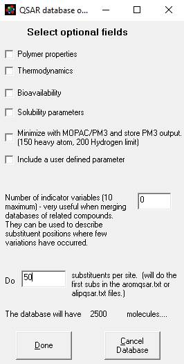
Make QSAR database from the molecule
This is the best and fastest option for creating a
database for classical QSAR analysis. It
is the only database creation option which incorporates typical Hansch substituent parameters (pi, MR, sigma, Verloop sterimol parameters) into the data. This routine is
otherwise somewhat more limited in what molecular properties it stores. It automatically stores molecular weight,
volume, connectivity and valence indices 1-4, HLB and Hansen's 3-D solubility
parameters. It also saves SMILES
structures and molecular formula.
Optionally you can store the 11 Joback and
Reid thermodynamic properties and the van Krevelen
type polymer calculations that MOLECULAR MODELING PRO
It will calculate the Lipinsky
bioavailability parameters (polar surface area, Moriguchi
Log P, hydrogen bond numbers) when the Bioavailability box is checked. It will calculate a number of properties
associated with solubility (Abraham solvation parameters, Log kow (MMP method), van Krevelen
3-D solubility parameters) and surfactants (HLB, viscosity) if the Solubility
parameters box is checked. If the
Minimize box is checked it will run a MOPAC PM3 geometry minimization and also
save some properties calculated by MOPAC like HOMO, LUMO, heat of formation and
ionization potential.
You may also create up to 10 indicator
variables. You can only vary one, two or
three substituent sites widely and 1-10 more sites in small ways with the
indicator variables.
Note that if you modify three substituent sites,
large databases can be created quickly.
We recommend you limit three substituent databases to no more than the
first 30 substituents in the alipqsar.txt and aromqsar.txt files. A 27000 molecule database would be created if you select 30
molecules (30 cubed). In the example
below. a two substituent site database generates 50x50 =2500 molecules.
The
reason this method can create fairly large databases quickly, is that only one
molecule has to be drawn. Draw the
template molecule, minus any substituents other than hydrogen. Then select this option. Click on one, two or three substituent sites
(or hydrogens to be replaced by substituents) when prompted by the
program. The program will determine
whether the site is aromatic or aliphatic.
You also must select the name and directory of the database file. It is possible to merge the newly created
molecules into an existing database.
This makes it possible to vary more than two substituent sites. The program will ask you whether you want to
merge the data or not if you choose to save the data to an existing file. If you only vary one substituent site you
also will be asked to choose the first three letters of the connection table
file names. This feature is there for
handy file erasing at a later time (e.g.
If you are
varying one substituent, then MOLECULAR MODELING PRO
Indicator
variables are particularly useful for substituent sites where you will have
very few differences. For instance if
you have a site that only uses hydrogen and chlorine as substituents you may
want to create an indicator variable for chlorine. The values would be 0 for hydrogen and 1 for
chlorine. If you then create a database
where you widely vary two other sites you can create the database varying all
three sites by first constructing the substructure to hydrogen and running the
database creation program as usual, but instructing the program to create 1
indicator variable. Then after the
database is created, change the hydrogen to chlorine and run the QSAR database
creation routine again, this time merging the data instead of creating a new
database. If you have three substituent
types at the same position (say H, F and Cl) you probably should create two
indicator variables - one for F and one for Cl.
You could, perhaps have an indicator variable that is not only 1 or 0
too, for instance in a polymer system, the variable could be number of monomer
units and two indicator variables could take care of different monomers in a
copolymer.
The program does a quick conformational analysis
when adding the substituents to the substructure. It checks for the conformation with the
lowest unbonded atom overlap and also checks for positive contributions from
hydrogen bonds at 30 degree rotational increments. This should result in a roughly optimized
molecule geometry. Some additional
optimization could be obtained by minimizing all the molecule in the directory
by checking the MOPAC option in the Options window above.
SMILES Notation from all molecules in a directory
Creates a list of SMILES structures in an ASCII file
called "Smiles.txt" for all the molecules in a directory. Each line contains one SMILES structure.
Print molecule
Print Graphics
Draws a black and white or color image to the
printer. The quality of this image is
likely to be better than the screen print below. The options selected for current screen
display will be used with the printer.
Screen Print
Does a screen print using an on-line printer in
color (if supported by the printer).
Entire
Directory (.Dat, .Mol)
All the molecules (*.dat,
*.mol) in the selected directory will be printed to the local printer (select
with the WINDOWS Control Panel/Printers).
The print out will be in black and white and will include the molecule
name. An example of the output is
Appendix 2 of this manual.
Allows you to change the
links (file locations) for cooperating
programs like NotePad, ChemSite, MOPAC and
RASWIN.
Exit
Quits the MOLECULAR MODELING PRO
Edit
Copy to clipboard
MDL Molfile
Copies an MDL Molfile to
the text portion of the clipboard. The
Paste MDL Molfile from Clipboard menu item will take this
connection table and input it as a new molecule. This molfile can be
used by a number of other programs and internet applications.
Graphics
Does a screen print to the clipboard. This picture can be used by any WINDOWS
program which can paste in a bit map.
For instance, in Microsoft WORD for WINDOWS position your cursor to
where you want to add the picture, select
paste from the edit menu and the bit map should appear in your
document. You might have to clear the clipboard contents before this will work.
CML - copies the structure to
the text portion of the clipboard using the CML (Chemical Markup Language)
format. For more information on this
format see http://www.xml-cml.org .
Paste from clipboard
MDL Molfile
Pastes an MDL Molfile from
the text portion of the clipboard into Molecular Modeling Pro Plus. Other programs, such as Chemsite
and Chemistry 4-D Draw are capable of placing Molfiles
on the clipboard.
Graphics
Pastes the current graphics on the clipboard onto
the Molecular Modeling Pro Plus screen
CML - pastes the structure from
the text portion of the clipboard using the CML (Chemical Markup Language)
format. For more information on this
format see http://www.xml-cml.org .
Clone molecule
Selection of this item will cause the program to
copy a molecule. If there is more than
one molecule on the screen, the user chooses the molecule to copy from a menu
of molecule names.
Delete molecule
Selection of this item initiates deletion of a
single molecule. The user select the
molecule to delete from a menu of molecule names.
Insert Text
After selecting this item, the viewer clicks on the
screen to insert text there. Text will
begin below the place clicked on. The
viewer types his text onto the screen.
Text font size and color is controlled with the Draw/Fontsize
and Draw/Color/ Set text color options.
You can display a title and up to
10 bulletted text items anywhere on the screen. Select the font and font color with the
routines under the Format menu. Then
select this item and follow the instructions.
You may wish to return the font to Microsoft Sans Serif, size 8.5 (the
default).
Name the molecule
Assigns a name to the molecule.
Format
Font
Changes the font, font size, font color for the
screen or printer.
Set background
color
The user selects the background color by clicking on
a color, or selecting some custom color.
Set text
color
Click on a color to set the text, frame, arrow and
graphics objects colors. Also determines
the colors of the sticks in ball and stick models.
Make molecule
a color
The user selects the color of one of the molecules
by clicking on a color. This option is
especially useful for docking two molecules on each other.
Color molecule
by charge
Colors atoms by partial charges:
blue:
most positive
green:
somewhat positive
white:
neutral
yellow: somewhat negative
red: most
negative
If the rotation option is set to rotate only one
molecule, then the user is asked to select which molecule to color. This makes it possible to color one molecule on
the screen by charge, and other molecules by normal color or lipophilicity.
Color molecule
by lipophilicity
Colors atoms by lipophilicity.
Calculates this value based on the HLB concept (regions of water and oil solubility):
dark
blue: most lipid soluble
light
blue: somewhat lipid soluble
white:
intermediate
light
bright red: somewhat water soluble
dark red:
most water soluble
If the rotation option is set to rotate only one
molecule, then the user is asked to select which molecule to color. This makes it possible to color one molecule
on the screen by lipophilicity, and other molecules by normal color or charge.
Color molecule
by residue
The molecules will be colored by residue. This works with molecules read in from
Brookhaven pdb files, MACROMODEL files which contain
this information, or molecules created with the amino acid or monomer
tools. If there are multiple molecules
present, the different molecules will also get different colors.
Restore molecule colors
Restores molecules to default atom colors.
Set atom color
Click on a color or choose a custom color for an
atom type (e.g. carbon normally green).
Changes will be registered in the file Moldat.txt and will be saved for
future use until you change the color again. If you changed carbon to gray,
then all carbon atoms will be colored gray unless changed with one of the
options above.
Size by charge
The atoms in the molecules will be sized by partial
charge after selecting this option. If
you have calculated
radius in angstroms =
Abs(atomic partial charge * 10)
where charge = 1 if on average the
atom is cationic and missing an electron,
-1 if anionic, and some fraction of 1 normally.
Tools
Reactor (Reaction
editor)
The reaction and mixture editor has two
functions. First, some stoichiometric calculations can be performed, such as predicting the amount of
product or determining whether the reaction proportions are balanced. Second, the editor is a simplified way of
arranging the molecules in a drawing of the reaction. The functions of the reaction editor are:
a) a "Main" spreadsheet grid contains the
names of the molecules, whether they are reactant, intermediate, or product, the molecular weight, ratio
added, moles added and grams added or obtained in the reaction. Editing these columns has the following
effects:
I) changing the name of molecule will change the
name used throughout the MOLECULAR MODELING PRO
ii) double clicking or hitting any alphanumeric key
changes the result in the second column from starting material to intermediate
to product and back again.
iii) changing the molecular weight (MW) changes the
MW used throughout the program, including when the molecule is saved to a
database.
iv) changing the reaction proportions causes a
recalculation of the moles added and grams added/produced, as well as a
reevaluation of whether the reaction ratios are balanced.
v) changing the moles used/produced or grams
used/produced causes all of the moles and grams calculations for all molecules
to change to the correct amount based on the reaction ratios and molecular
weights. It also changes all the values
in the solution spread sheet.
b) a "Solution" spread sheet grid with the
following columns:
i) changing the name of
molecule will change the name used throughout the MOLECULAR MODELING PRO
ii) % (w/v) is the percent of the material per total
volume.
iii) ppm is the parts per million of the compound
(mg/L)
iv) molarity is the moles/liter of the compound
Changing any of fields ii-iv will cause the results for the other fields and
for the grams and moles fields in the Main spread sheet to change for this
compound.
c) a text box to indicate the total reaction
volume. Changing this number will also
change all the values in the "Solution" spread sheet.
d) Filling in the above and below arrow text boxes
will instruct the program what to type above and below the reaction arrow if
you hit the Draw button. The arrow 2
boxes only apply if you have an intermediate product designated.
e) Hitting the Done button quits the reaction
editor.
f) Hitting
the Draw button causes the program to draw the reaction as currently specified
in the spreadsheet. The reaction editor
is quit and the reaction drawn in the Drawing form. Print out the reaction with the
File/Print/Screen Print menu combination or save it as a bitmap.
g) The Print button will do a screen print of the
Reaction editor.
h) The Get button will get a reaction stored with
the Save button. Molecules currently in
memory are erased.
i) The Save button saves the
reaction molecules, and some features of the reaction such as identification of
starting materials and product, ratios, and arrow text.
j) The Units button allows you to change the units
of mass and volume displayed by the program.
Units of volume supported are hectoliters, liters, milliliters,
microliters, gallons and fluid ounces. Units
of mass supported are metric tons, kilograms, grams, milligrams, micrograms,
English tons, pounds and ounces.
k) The Info button brings up another panel of text
data. This data is stored and retrieved
with the reaction. The field are
molecule name, trade name, manufacturer,
l) The Props button covers the solution grid with
the properties grid. Hitting this button
again, swaps these grids again. Some
information on the total HLB of the mixtures of molecules appears below the
properties panel. The molecule name,
molecular volume, HLB and Hansen 3-D solubility parameter for each molecule are displayed in
the properties grid. Changing the
mixture ratio in the Main grid will change the total HLB values displayed in
the total properties box.
Tutorial D covers the reaction editor in more
detail.
Add amino
acid
A small window appears with the 3 letter codes for
the various amino acids. Select the
geometry of the acid by clicking on one of the 4 buttons at the top, then click
on the amino acid code. The amino acid
selected will be drawn on the screen. If
you wish to connect it to a previously drawn molecule hit the “Connect” button
on the main drawing window, and click on the two atoms to be connected. If you would like the amino acid residues to
connect automatically then check the "Build polypeptide" box. After checking this
box, every time you select an amino acid it will be added to the chain. The amino group from the new residue is added
to the carbonyl from the last amino acid selected.
The geometry of the connections is set by selecting
the helix, sheet, turn or specify buttons.
The geometries are derived from measuring dihedral
angles in proteins:
Torsional bond helix sheeet turn specify
C-N-CO-C 180 180 180 you set
CO-C-N-CO 282 240 6 you set
N-CO-C-N 326 144 87 you set
You can also color the molecules already on the
screen and those to be drawn by this tool by residue, structural type, molecule
(subunit, chain), or by the normal colors.
Check boxes at the bottom of the amino acid tool window control these
coloring schemes. Each amino acid is
defined as a residue, so coloring by residue will give each amino acid or
monomer a different color. This works
with residues input from MacroModel or Brookhaven
files too. Coloring by structural type
(helix, sheet, turn or other) works with files input from the Brookhaven
protein database as well as with this tool.
The colors used are magenta for helices, yellow for sheets, blue for
turns and white for other.
Add monomer
A small window appears with the name of the polymer to be drawn. Some of these
names are abbreviations:
PET=polyethylene
terephthalate
Clicking on the "Build polymer" check box
and one of the monomers will cause the monomer to be automatically added to the
highest numbered atom of any existing molecule, as long as a valence is
free. The addition occurs at the lowest
numbered atom of the monomer added.
Addition of several monomers at once is possible by checking the
continuous addition check box and typing a number in the 'number of monomers'
text box. The atom limit for Molecular
Modeling Pro Plus is 4000.
Huckel Molecular Orbital Theory
A simple LCAO (linear combination of atomic
orbitals) method for the calculation of energy due to pi orbitals and
bonds. The partial charges, bond
strength, molecular stability and other properties can be estimated quickly in
conjugated and aromatic systems using this method. It assumes that the contributions of sigma
orbitals and bonds are negligible and so is not so useful for molecules high in
saturation. It also assumes that the
conjugated pi system is planar. It is
quite useful in predicting properties of different aromatic systems such as
benzene or naphthalene and conjugated systems such as butadiene.
MOLECULAR MODELING PRO
The option to used "extended" Huckel theory (also known as the Hoffman method) is
included with MOLECULAR MODELING PRO
References:
1. Andrew Streitwieser Jr., 1961,
"Molecular Orbital Theory for Organic Chemists,", John Wiley
and Sons,
2. K. Jeffrey
Johnson, 1980, "Numerical Methods in Chemistry", Marcel Dekker Inc.,
3. W.P.
Purcell and J.A. Singer, 1967, "A brief review and table of semiempirical
parameters used in the Huckel Molecular Orbital
Method", J. Chem.
4. N. Trinajstic, 1992, "Chemical Graph Theory",
5. R.
Hoffman, J. Chem. Phys. 39: 1397 (1963)
A semiempirical quantum chemistry program that I
have used in my research to calculate
partial charges and dipole moments.
Molecular
Modeling Pro Plus calculates partial charges and dipole moments using either
Eigenvalues (energy levels) for chloroethane:
-1.5104 -1.1402 -1.004 -.90667 -.8089 -.70532 -.63821 -.56419
1
2 3 4 5 6
7 8
-.51512
-.51362 .099803 .22428 .23891
.26694 .26879 .28066
9
10 11 12 13 14 15 16
.29986
.30499 .31842 .36986
.37868 .39477
17
18 19 20
21 22
The HOMO value in the above example is the last
negative value
(-0.51362).
There are 20 valence electrons in chloroethane, with two
electrons/orbital. Thus the tenth
eigenvalue is the HOMO (20 divided by 2 =10) and the eleventh eigenvalue is the
LUMO value (.099803).
If open shell is chosen, the results of the matrices
used in calculating the results are reported.
Consult a specialist in quantum mechanics to interpret these
results. If you have ionic species
present then use the Open shell method.
The partial charges and dipole moment are at the end of the file. The file is called "
You also have the option of using the INDO procedure
instead of
INDO is only parameterized for atoms with atomic
numbers less than 9, so cannot be used for molecules with P, S or Cl in
them. If you want to obtain coupling
constants for the atoms in a molecule, than INDO will list this result with the
partial charges at the end of the file.
After running
If you use
During the batch creation of a database of all
MACROMODEL files in a directory, if you check the "Use
Charge can also be used to calculate the log octanol
water partition coefficient (log P, Log Kow) . A method was recently
published by K.F. Moschner and A. Cece
(1995) that used Gasteiger-Huckel charges and other
atomic properties to calculate Log Kow. We have modified this method to work with
Calculating dipole moments from the Calculate menu
uses the modified DelRe method, not
For more on
J. Pople and D. Beveridge,
Approximate Molecular Orbital Theory, Mc
Graw-Hill, 1970.
J. Pople and G.A. Segal,
J. Chem. Phys., 43: 8136 (1965)
J. Pople and G.A. Segal,
J. Chem. Phys., 44: 3289 (1966)
D.P. Santry and G.A. Segal,
J. Chem. Phys., 47:158 (1967)
Raymond Daudel, Georges
Leroy, Daniel Peeters and Michel Sana, Quantum Chemistry, John Wiley and Sons,
For a historical overview of the development of self consistent field theory,
The log P method referred to is in Environmental
Toxicology and Risk Assessment - Third Volume,
A public domain version of MOPAC version 6 is
included with MOLECULAR MODELING PRO
MOPAC should interact with
MOLECULAR MODELING PRO
Executable File = “c:\ your
MOLECULAR MODELING PRO
Input File Name =
"c:\your MOLECULAR MODELING PRO
Output File Name =”c:\your
MOLECULAR MODELING PRO
These links are stored in
the file moldat.txt.
After the links are set up,
you will be able to run MOPAC from within the MOLECULAR MODELING PRO
Using MOPAC with charged
species: MOLECULAR MODELING PRO
Atom
types supported by MOPAC v. 6 methods:
MINDO: H, C, N, O, F, P, S, Cl
AM1: H, B, C, N, O, F, Na, Al, Si, P, S, Cl, K, Zn, Ge, Br, I, Hg
PM3: H, C, N, O, F, Na, Mg, Al, Si, P, S, Cl, K, Zn, Ga, Ge, As, Se, Br, Cd,
In, Sn, Sb, Te, I, Hg, Tl, Pb, Bi
Key
words accessed through the Check Boxes
·
1SCF - Does one SCF (self consistent field)
and quits. Good to use if your geometry
is already optimized and you just want to print out charges and dipole.
·
GEO OK - allows very short bond lengths as in a hydrogen molecule (H2)
·
PRECISE - increases the precision of the calculations a hundred fold.
·
DENSITY - causes the final density matrix to be printed out.
·
BONDS - prints out the final bond order matrix - useful in determining bond
strength. The diagonal of the matrix
contains the atomic valences.
·
FORCE - The force constants for the molecule are printed out as well as
the moments of inertia.
·
SYMMETRY - the user types in
SYMMETRY constraints. Consult the MOPAC
manual for more information. In the
example below, two symmetry constraints are defined, both involving atom number
3. In the first symmetry contraint atom 3 is
constrained by type 1 (bond length set equal to the reference bond length) with
the reference being atom 5. In the
second constraint, atom 3 is constrained by type 2 (bond angle equal to the
reference bond angle) with the reference being atom 5 once again. This sets the two hydrogens as equivalents.
Example
- file created with SYMMETRY key word for fomaldehyde
SYMMETRY T=3600
molecule 1
MOPAC calculations:
O
C
001.1062 1
H
001.1062 1 123.5152
1
XX 001.6090
1 109.4712 1
180.0000 1 3
2 1
H
001.1062 1 112.9740
1 000.0000 1
2 3 4
XX 002.0920
1 123.4915 1
180.0000 1 2
3 4
0 0.00 0 0.00 0 0.00 0 0 0 0
3 1 5
3 2 5
·
THERMO - Thermodynamics calculations can be performed on
molecules. The key words FORCE and ROT
also must be included. The combination of these three key words will give the
user additional thermodynamic property calculations: internal energy, heat capacity, partition function and entropy for translation, rotation and
vibrational energy over a range of temperatures.
·
VECTORS - Prints out the eighenvectors.
·
ROT = n (where n = the symmetry number of the molecule). Examples of
symmetry numbers:
C1 CI
CS 1 D2 D2D D2H 4 C(
C2 C2V C2H 2 D3
D3D D3H 6 D(
C3 C3V
C3H 3 D4
D4D D4H 8 T TD 12
C4 C4V C4H 4 D6
D6D D6H 12 OH 24
C6 C6V C6H 6 S6 3
ROT is a necessary key word
for thermodynamics calculations (see THERMO above)
·
UHF - The unrestricted Hartree-Fock Hamiltonian is used.
·
POLAR - the polarizability and first and second
hyperpolarizabilities are to be calculated.
·
List reaction Coordinates - the user will be prompted for a reaction center
and reaction coordinates (see MOPAC manual for explanation)
Some
other MOPAC key words
Many of the MOPAC key words
are handled by MOLECULAR MODELING PRO
·
BIRADICAL - some biradical molecules will not optimize without this
keyword. MOLECULAR MODELING PRO
·
DENOUT - prints a density matrix file out for use by the QCPE program
DENSITY.
·
ISOTOPE - Prints out the Force matrix to a file for use by some
programs.
·
MECI - prints out the details of the Multi Electron Configuration
Interaction. If you also check VECTORS
it will print the state vectors.
·
SADDLE - determines a transition state - not fully supported by
Molecular Modeling Pro Plus yet.
More
uses of MOPAC
MOPAC has many additional
capabilities. For instance, to find
homolytic bond dissociation energies calculate the heat of
formation of the parent molecule and the two fragments formed by breaking the
bond. Subtract the heat of formation of
the parent from the sum of the heat of formation of the two fragments. Make sure you add the charges to the the ionic fragments (+ and – buttons at lower left of the
drawing window). By following this MOPAC
procedure for all the bonds in a molecule, the least stable bond can be
determined. An automated process has
been added to MMP Plus to calculate the bond dissociation energy for all the
bonds in a molecule. Numerous other useful methods are described in the
literature and can be found by an internet search.
The Image Processor is a tool for enhancing images
and saving them as WINDOWS bitmaps, JPEG files and HTML web pages. It includes a Java Script generator that
allows you to depict rotating molecules within an HTML web page.
The Image Processor is accessed through the Tools
menu.
The Image Processor Window appears after selecting
the menu item. In it is the currently
drawn molecule and any other graphics depicted in the Drawing Window. From the Edit menu of the Image Processor you
can crop an image, resize an image, adjust its brightness and contrast and add
text. You can overlay one image on top
of another with user selected transparency from the Edit window. From the File menu of the Image Processor
window you can Open and Save Images in bitmap or JPEG format.
Also from the File menu you can create HTML
pages. Before creating an HTML page add
text, crop and adjust brightness and contrast.
Here are instructions for creating a web page contatining
a rotating image.
1) Draw the molecule in the drawing screen.
2) Select the Image Processor from the Tools menu.
3) Add text to the drawing in the Image Processor
Window. Select "Add Text" from
the Edit menu. Type in the text in the
Text Editor. Click on the Font button
and select the font and font size you desire.
Hit the Done button. Hold down
the left mouse button and drag the text to where you want it. Do not worry about the image being covered
up. When the text is where you want it,
release the left mouse button. If you do
not like the result, hit the Undo button on the Edit menu.
4) Choose "Crop" from the bottom of the Edit
menu. Draw the box around the part of
the image you want to keep with the mouse.
To do push down the left mouse button at the upper left corner and drag
the cursor to the lower right corner while holding the mouse button down. Release the button at the lower right corner.
5) Choose "Save as HTML" from the File
menu. When prompted choose a file name
for the HTML page.
6) The HTML Editor appears. This window allows you
to add corporate logos, a title, text above and below the main image, create a
rotating molecule, add buttons to the page and a mail link. All of what is described below is
optional. If you do nothing but hit the
"Done" and HTML page will be created with nothing more on it than
what appears in the Image Processor Window. From top to bottom of this window,
here is what you can do with this window.
a) You can
set the background color for the entire page from the Options menu at the top
of the HTML Editing window.
b) In the
text box labeled "URL for logo graphics at the top" you can place a
link to an image of your corporate or university logo. For example if you place this image in the
subdirectory /gif and the logo graphics file is named mycollege.gif you would
type in gif/mycollege.gif in this box.
If left blank, the program will ignore this part of the HTML page
creation.
c)
"Title of Page": Type
in the Title. Select the font button to
change the background color for the title, the text color, the font and the
font size. The Title appears between the
corporate logo graphics and any text you type in above the main image.
d) "Link
(URL) to attach to the Drawing". If
you assign a link, then clicking on the main image will send the user to the
designated URL. For instance, if you
type "http://www.norgwyn.com" here then clicking on the main image of
the molecule will send one to the Norgwyn Montgomery
Software home page.
e) "Text
above drawing". You can type in
text here that will appear above the drawing of the molecule, for instance a
description of its use. The font, font
size, font color and font background color can be selected by clicking the
"Font" button to the right of the text box.
f) "Text below drawing": Places text below the image. Click on Font to change the font.
g) "Add
these links to the bottom of the page":
This adds buttons to the bottom of the page which when clicked will send
the user to some other URL. For
Instance, typing "HOME" in the captions column and
"http://www.norgwyn.com" in the URL column will place at button below
the image and text labeled "HOME" that when clicked will send one to
the Norgwyn Montgomery Software home page. You can add several buttons.
h) If you want a mail link on the page, check the
check box and type in the e-mail address.
i) "Animate
Molecule" check box. If you check
this, Java Script will be written that makes the molecule depicted in the image
rotate around the Y axis. Speed of
rotation is a function of image size (the smaller the faster it rotates). The molecule Display mode will be the one
selected in the Drawing window.
Make
substructure keys
This option creates a substructure keys file for all
molecules in a directory (*.dat, *.mol) for use with
the substructure and reaction search options in the Calculate menu and stores
the result in a file called MMP.SSF in the directory that the connection tables
are in. The substructure keys file is
actually another database that can be used for modeling physical
properties. The 118 keys and 10
molecular properties stored in the ssf file can be
read into a statistical program, combined with experimental values and analyzed
with PLS or another regression technique to come up with a model. See the database tutorial part 17 for more
information.
Substructure Search
Draw a template substructure to the screen. Then select this option. The program searches the substructure keys
file in the directory chosen for similar number of atoms and similar key
fragments with the keys for your substructure.
If the directory does not contain a keys file then the program must
first create one (this will take a little time). After doing this, the program will ask you if
you want to make a more exhaustive search.
If you answer yes, the program will search all the connection tables
pointed to by the keys file to make sure that all the atoms included in the
substructure drawn on the screen are matched.
Note that this could take some time if your directory contains thousands
of compounds. The list of molecules
found to match is displayed. You may
select a molecule from the list to edit or analyze. The list stays in memory and can be displayed
again with the Show Search Results option below. The maximum number of hits found can be 2500,
but the number of compounds searched is limited by memory only.
Reaction
Search
Draw a template substructure to the screen. Then select this option. The program searches the substructure keys
file in the directory chosen for similar number of atoms and similar key
fragments with the keys for your substructure.
If the directory does not contain a keys file then the program must
first create one (this will take a little time). The program then goes through all of the
reaction file (*.rct) to see if any of the matched
molecules are contained in the reactions in the directory. If so, the names of the reactions are
displayed. You can select one of the
reaction for analysis or editing. The
list of matches stays in memory and can be displayed again with the Show Search
Results option below.
Similarity Search
Draw a molecule on the screen. A screen containing some options will
appear. Choose the percent similarity
minimum that you wish. If you get too
many or too few hits, you may want to rerun the search with a higher or lower
value. You can also pre-filter data for
a range of molecular weights or a range of % hydrophilic surfaces. For instance if you only want small
lipophilic molecules, you could set the maximum molecular weight to 200 and the
maximum % hydrophilic surface area to 25.
The program will then search
a SSF file of your choosing for similarity of your molecule to all the
molecules in the file. It uses the keys
used in substructure searching plus the 1,2 and 3 connectivity and valence
indices, the kappa 2 shape index, molecular volume and percent hydrophilic
surface for determining similarity. The
results are displayed in a list at the end of the search and also by the Show
Search Results option below.
Show
Search Results
This option displays the matches from the Substructure
Search, Reaction Search or Similarity Search menu items above. Clicking on one of the matches and the
Display button will display the molecule or reaction selected in the list. Clicking on the Print button will print out
drawings of all the structures in the list with their names. You can delete a molecule from the list with
the Delete button so it will not be printed out.
Rotate
X
Rotates one or all of the molecules on the screen
along the x axis. The user can type in a
value in the text box and select the DONE button to rotate the molecule by a
specific amount. Secondly, the user can
simply select the DONE button without typing to rotate the molecule 90
degrees. Thirdly, the user can select
AUTOROTATE to start the molecule rotating.
This activates the X, Y, Z, Quit, Stop, Trans z, <, and > buttons
which are described below.
Rotate command
buttons:
Quit: Ends
the rotation routine and reactivates the Rotate menu.
X: Changes
the rotation to the x axis, and starts the molecule rotating.
Y: Changes
the rotation to the y axis, and starts the molecule rotating.
Z: Changes
the rotation to the z axis and starts the molecule rotating
Reverse:
Reverses the direction of x,y, or z rotation
or z translation.
>:
Increases the angular interval and thus speeds the apparent speed of
rotation. The default angle is 5
degrees. Each time > button is hit,
the interval doubles.
<:
Decreases the angular interval and thus slows the apparent speed of
rotation. Each time the < button is
hit, the interval is halved.
Trans z: This button is visible only
when Perspective or Clipping is selected from the Display menu. It changes the z coordinates of the rotating
molecules and stops the rotation. In
other words, it moves the molecules in or out of the screen.
Stop: Stops
rotations and translations, without leaving the rotation routine.
While the rotation options are activated, it is possible
to perform most of the other MOLECULAR MODELING PRO
Y
Acts like the X button, but rotates one or all
molecules along the y axis.
Z
Acts like the Y button, but rotates one or all
molecules along the z axis.
Bond
Rotates a bond.
The user selects the two atoms to rotate by clicking on them when
requested. If there are less than four
consecutive atoms in a molecule, no rotation is possible and the program does
not execute this routine. The program
will also refuse to rotate a ring bond.
As with other rotation options, the user can type in the desired degrees
of rotation in the text box by changing the 90 to the desired angle and
selecting DONE. Alternatively, the user
can select AUTOROTATE which will start the bond rotating and activate the
following command buttons and features:
Quit: Ends
the bond rotation routine and reactivates the Rotate menu.
Reverse:
Reverses the direction of bond rotation.
>:
Increases the angular interval and thus speeds the apparent speed of
rotation. The default angle is 5
degrees. Each time > button is hit,
the interval doubles.
<:
Decreases the angular interval and thus slows the apparent speed of
rotation. Each time the < button is
hit, the interval is halved.
Strain: This button turns on and off a
routine which calculates increases in energy due to atom overlap of rotating
atoms, coulombic charge interactions or going through torsional barriers. The strain is in
kcal/mole. Low energies are preferred
conformations. The atom overlap routine
is from the minimizer in MOLY. The
torsional barriers are, and are limited to combinations of O, N, S,
C=C,C=N,C=O,C=S, aromatic ring, or a default value for everything else. Extended conjugations are not searched for
(it searches for bonds and atoms adjacent to the two atoms attached to the
rotating bonds), so torsional barriers may be slightly overestimated. The result is displayed in a box at the top
of the screen. If two molecules overlap,
the unbonded strain will reflect this.
If you do not want to include intermolecular strain then move the
molecule whose bond is rotating away from the other molecules.
Stop: Stops
rotations without quitting the rotation routine. This makes it convenient to make a change in
the molecule or perform some other operation and then resume bond rotation.
In addition, the function of the interatomic
distance, angle and dihedral angle routines (under the Calculate menu) change
when bond rotation is selected. The
values are continuously updated in a box while the molecule rotates. This is way the dihedral angle of an atom
attached to the rotating bond can be monitored.
Rotation Options
The user specifies by clicking on check boxes,
whether the x, y and z rotations apply to one molecule or all of them. In addition,
the user selects if the axis of x, y or z rotation is determined by the
center of the molecule or the center of the screen. Selecting center of the molecule usually
gives the best result. However if the orientation of two molecules to each
other is important, then select center of the screen.
Calculate
Note on calculations: The calculations vary in reliability. You may want to consult the literature
references listed to get an idea of the training sets used in calculating a
property. If your molecule does not
resemble the molecule in the training set, then its predicted property is less
likely to be correct. One logical way to
correct for property miscalculations is if you have an experimental value for a
related compound, draw in the related compound and predict its property. Then add the difference between the
experimental and predicted value to the molecules for which you wish to
calculate values. A table listing
reliability of some of the properties is found near the end of this manual.
Interatomic distance
The user clicks on any two molecules on the screen
when requested. The program returns the
distance between the atoms in angstroms.
The display is either in a message box, or, if the bond rotate routine
is in effect, displays the value in a text box at the top of the screen which
is updated as the bond rotates.
Incidentally, here are some of the references used
to determine the correct bond lengths:
1)
2) The bond order-bond length relationship by J.P. Paolini (J. Computational Chem., 11: 1160-1163
3) Valency and Molecular Structure, Fourth
edition, by F. Cartmell and G.W.A. Fowles,
Butterworths (from this was found, besides bond lengths for various pairs a
calculation method called the Schomaker-Stevenson
relationship which allows the calculation of bond lengths when they are not
known:
bond
length = r(a) + r(b) -0.09*(difference in electronegativity)
where r(a) and r(b) are the covalent radii
of the atoms and electronegativity values of elements are
from Pauling.
Angle
Three atoms are clicked on (the center atom in the
angle is clicked on second) when requested by the program. The program will return the value in an
information box, or, if bond rotation is activated, will return the answer (in
degrees) in a text box at the top right and update the value as the bond
rotates.
Dihedral
angle
Four atoms are clicked on when requested by the
program. The program will return the
value in an information box, or, if bond rotation is activated, will return the
answer (in degrees) in a text box at the top right and update the value as the
bond rotates. The dihedral angle is the
angle formed between the plane formed by the atoms selected first, second and
third and the plane formed by atoms 2,3 and 4.
Molecular weight
The molecular weight of all of the molecules is
supplied in a box. This property is as
exact as the atomic weights reported in the literature.
Molecular volume/density
The molecular volume in cubic angstroms is displayed
for all of the molecules. Volume is calculated
using the method of A. Bondi (J. Phys. Chem. 68:441), 1964. The program also calculates surface area using the same elementary 3-D geometry principles and calculates
density. Density is calculated by
dividing molecular weight by volume and then correcting for fragments found
with an algorithm I derived from solvents.
Individual volumes and surface contributions of each atom are also
listed.
Point charges/dipole moment
The partial charges are calculated using DelRe's method (G. Del
Re, J. Chem. Soc., (1958), 4031-4040; Biochem. et Biophys. Acta 75:153-182 (1963); D. Polland
and H. Sheraga, Biochemistry 6:3791-3800 (1967) and
partly with values obtained by trial and error on conformationally constrained
molecules with known dipole moments. The
partial charges of Del Re were further modified so that they too resulted in
dipole moments reported in the literature.
Some account of pi bond (as well as sigma bond) is taken into account by
MOLECULAR MODELING PRO
With version 3.1 two PEOE (partial equalization of
orbital electronegativity) methods are introduced for the calculation of
partial charge. The first of these
methods uses Gasteiger and Marsili’s
method for finding the sigma contribution and adds one quarter of the pi
contribution to charge calculated by Huckel
Theory. The second method (MPEOE) is an
attempt to improve on this method.
References:
*
Del Re method: G. Del Re, J. Chem. Soc. 4031
(1958); Poland and Scheraga,
Biochemistry 6: 3791 (1967); Coefficients modified in MOLECULAR MODELING PRO
*
PEOE method: J. Gasteiger and M. Marsili,
Tetrahedron 36:3219 (1980).
*
MPEOE (DQP) method: K.T. No, J.A.
Grant and H.A. Scheraga, J. Phys. Chem. 94:4732
(1990) and K.T. No, J.A. Grant, M.S. Jhou and H.A. Scheraga, J. Phys. Chem. 94: 4740 (1990); J.M. Park, K.T.
No, M.S. Jhou and H.A. Scheraga,
J. Comp. Chem. 14:1482 (1993).
Dimensions
This operation displays three values for all of the
molecules: the length along the x axis, the width along the y axis and the depth along the z axis in angstroms.
After this the user is asked if he would like to do some time-consuming
calculation involving dimensions. First
you will be asked if you would like to calculate the global maximum and minimum
dimensions. If so, the molecule will be
rotated in 5 degree increments along the y and z axes for 360 degrees and the
maximum and minimum dimensions found will be reported. Then you will be asked if you want to orient
the maximum dimension along the x axis.
If you answer yes to this you will also be given the option of finding
and orienting the molecule’s maximum width along the y axis (the maximum length remains on x).
Solubility parameters
The program returns the following values for all
molecules as a Microsoft Notepad file:
Log P: an estimation of the log of
the octanol/water partition coefficient using fragment and atom constants after
the method described in C. Hansch and A. Leo's 1979
compendium. This measure of solubility
is used with moderate sized molecules such as typical pharmaceuticals or
pesticides. Most, but not all of the
values for fragments are from Hansch and Leo's book.
Reference: Substituent Constants for Correlation Analysis in Chemistry and Biology
by C. Hansch and A. Leo (1979), Wiley and Sons.
Ghose and
Crippen’s Log P: There is a second method of calculating log P based on summing
contributions of atom types, instead of fragments. This method was published in 1988 in J. Chem. Inf. Comput.
Sci. 29: 163-172.
Here, for instance, is an example of how this
calculation is made for n-propanol:
atomic
Description hydrophobe refraction
carbons
CH3R, CH4 -0.6771 2.9680
CH2R2 -0.4873 2.9116
CH2RX -0.8370 2.9244
oxygen
alcohol 0.1402 1.7646
hydrogen
H on C(0) sp3 0.4418 0.8447
H on C(1) sp3 0.3343 0.8939
H on heteroatoms -0.3260 0.8000
where X is a
heteroatom including oxygen, R is an attachment through carbon, and C(0) is carbon with no electronegative
atoms and C(1) is carbon with 1 electronegative atom.
Log P for propanol =
-0.6771 - 0.4870 - 0.8370 + 0.1402
+
5(0.4418)+2(0.3343) - 0.3260
Molar refractivity (MR) is calculated by summing the atomic refraction values in the same way.
Reference: V.N. Viswanadhan,
A.K. Ghose, G.R. Revankar and R.K. Robins, 1988, J.
Chem. Inf. Comput. Sci., 29: 163-172.
QLogP, Hydrogen bonding, Steric
hindrance and enzymatic hydrolysis models:
The idea for these algorithims
comes from two papers by Nicholas Bodor and Peter
Buchwald. Their goal was to be able to
reliably predict enzymatic hydrolysis.
Looking at a number of different factors they found Log octanol water
partition coefficient, the steric hindrance of the double bonded oxygen
involved in the hydrolysis and the partial charge on the carbon to which the
oxygen is attached to be correlated adequately to give a good predictive model. They also developed a new method for
calculating Log octanol water partition coefficient which they dubbed QLogP which uses a very simple two variable underlying
model. The two factors which they use to
calculate Log P with are hydrogen bonding (from a table of values given in the
paper) and van der Waal’s volume. Our
results are very similar, but slightly different from theirs because MOLECULAR
MODELING PRO
HLB: hydrophilic-lipophilic balance. Roughly, this value is
obtained by dividing the molecular weight of the water soluble portion of the
molecule by the totalmolecular weight of the molecule
and multiplying the result by 20. There
are some additional fragment and atom based factors calculated also. For instance, sodium, potassium or phosphate
groups add a large constant to the number, so that results higher than 20 are
possible. In addition, some combinations
of halogens can make the HLB be less than 0 if volume based calculations are
used instead of molecular weight.
Finally, in an attempt to use HLB for non-surfactant molecules, I have
added some fragment modifications not reported in the literature for fragments
with several adjacent functional groups.
The HLB concept is used primarily
for surfactants and formulations work.
The method here could be referred to as a modification of the method of
solubility
parameter: Materials with like solubility
should dissolve in like. This measure of
solubility is in the units (delta/(MPa)^0.5).
It is calculated here by taking the square root of the sum of squares of
dispersion, polarity and hydrogen bonding (the Hansen 3-D solubility parameters). The reference for the
calculation of the solubility parameter, dispersion, polarity and hydrogen
bonding is the Handbook of Solubility
Parameters and Other Parameters by Allan F.M. Barton,
dispersion: (Hansen 3-D parameter) a measure of repulsive forces between
molecules (the tendency to disperse)
polarity: (Hansen 3-D parameter) a measure of polarity of the molecules. Molecules with localized positive and
negative regions are said to be polar.
hydrogen
bonding: (Hansen 3-D parameter) a measure of the tendency of a molecule to
form hydrogen bonds.
hydration
number: the number of water molecules
bound to the molecule in solution.
reference: McGowan, Tenside
Surfactants 27: 229-230 (1990)
hydrophilic
surface area: the surface area that binds
water instead of repelling it.
% hydrophilic
surface area: the percentage of the surface area of the
molecule that is hydrophilic.
Polar surface area yields the surface area occupied by nitrogens and oxygens (and hydrogens attached to N and O) in a molecule, using the group contribution method outlined in the paper, P. Ertl, B. Rohde, P. Selzer, Fast Calculation of Molecular Polar Surface Area as a Sum of Fragment-based Contributions and Its Application to the Prediction of Drug Transport Properties, J.Med.Chem. 43: 3714-3717 (2000). It calculates a value for both charged and uncharged O and N. Polar surface area has been found useful for drug transport modeling including intestinal absorption and penetration of the blood-brain barrier. The authors of the paper cited call their method of calculations Topological polar surface area or TPSA.
Surface
tension in dynes/cm. This method was obtained from the Handbook of Chemical Property Estimation
Methods. It has only been tested
against small solvent molecules. It is
determined from the boiling point and density of the molecule and inaccuracies
in the calculations of those two physical properties will be carried over to
the surface tension calculation.
water
solubility: The water solubility method
comes from G. Klopman, S. Wang and D.M. Balthasar, J.
Chem. Inf. Comput. Sci. 32:474-482 (1992). MOLECULAR MODELING PRO
A method devised by
Log
S = -Log P - 0.01*(25-MP) + 0.8
Values derived from both the fragment based Log P
calculation and the Crippen atom-based calculation are given.
An algorithm was also designed by the author to
calculate log water The method for calculating water solubility is included in
the sample program "Display" included with MOLECULAR MODELING PRO
Log molar
olive oil/gas partition coefficient
The partition coefficient between olive oil and air
is calculated based on the method of Klopman et.al.
(J. Chem. Inf. Comput. Sci. 37:569). Handles common organic atom types (but not
P). This method is useful for predicting
the loss of a compound from an oily substance into the atmosphere.
Solvation Parameters (After Abraham)
Solvation
parameters (developed by Abraham's group, references 1, 2, 3, 5, 6) are widely used
to construct models for determining partition coefficients of molecules from
structure. Selecting this item from the
Calculate menu brings up the following Window.
This table contains descriptors for the currently drawn molecule and a
separate larger table with model coefficients and predictions from the
literature. The Result for the model is made by multiplying the descriptor of
your drawn molecule with the corresponding model coefficients and adding these
terms together: Result = intercept + e*E + s*S + a*A + b*B +v*V (for
partitioning of your molecule in a water/solvent system)
Or:
Result=intercept+e*E + s*S + a*A + b*B +l*L (for partitioning of
your molecule in an air/solvent system)
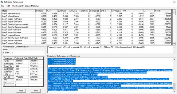
The
table at the top are the multiple regression coefficients for the models.
The
table on the left are the parameters for the current molecule that will be
multiplied with the coefficients.
The
left table values were obtained by adding together values for the fragments
contained in the molecule. These
fragment values can be found in the files solvation\solvationA.csv and
solvation\solvation_SumA2H.txt.
Parameter
Descriptions:.
R2
(called E in most papers) is the excess molar refraction (i.e. the molar
refraction of the solute minus the molar refraction of an alkane of equivalent
volume.)
SumPi2H
is a combined dipolarity/polarizability descriptor
(called S in some papers.)
SumA2H
is the overall hydrogen bond acidity (sometimes called A.)
SumB2H
is the overall hydrogen bond basicity (somtimes
called B.)
SumB20
is an alternative overall hydrogen bond basicity used in calculation of solvent:solvent systems.
L16
is the log of the solute gas-hexadecane partition coefficient.
Vx
is the McGowan characteristic volume in cm^3/mol divided by 100.
A*B
is the interaction between hydrogen bond acceptors and donors obtained by
multiplying them together.
The
Result is obtained by adding the components together:
Result
= Intercept + a*R2 + b*SumPi2 + c*SumA2H + d*SumB2H + e*SumB20 + f*L16 +
g*Vx/100 + h*A*B
where
a, b, c, etc. are the values from the table above and R2, SumPi2 etc. are from
the table at the left.
Models
are stored in a text file called solvation\solvation_modelsA.csv. You can add
more models from the Edit menu of this window.
Alternative
models without an intercept are stored in a text file called
Abraham_NoIntercept.csv. There are over
290 solvents modeled there and you can load this file from the File menu of
this window.
Log
P values are the partition coefficients for compounds in two solvent
systems. Log K values are the
coefficients of solubility from a gas phase to a liquid phase or coefficients
for biological activity.
All
values are at 290 K except for the biological values Log K and thresholds which
are at 310 K.
The
units for biological thresholds are ppm (vol:vol).
References:
1.
James A. Platts, Darko Butina, Michael H. Abraham and
Anne Hersey, 'Estimation of Molecular Free Energy Relation Descriptors Using a
Group Contribution Approach', J. Chem. Inf. Comput.
Sci. 1999, 39, 835-845. The lists of
descriptors can be found in the files 'solvation\solvationA.csv' and
'solvation\solvation_SumA2H.txt' in your MMP directory.
2.
Yuan H. Zhao, Michael H. Abraham and Andreas M. Zissimos,
'Determination of McGowan Volumes for Ions and Correlations with van der Waals
Volumes,' J. Chem. Inf. Comput. Sci. 2003, 43,
1848-1854. The list of values used can
be found in the file mcGowan_Vx.txt in your MMP directory.
3.
Michael H. Abraham and Yuan H. Zhao, 'Determination of Solvation Descriptors
for Ionic Species: Hydrogen Bond Acidity and Basicity,' J. Org. Chem. 2004, 69,
4677-4685. The data was used to expand
the previously mentioned tables in your MMP directory.
4.
Michael H. Abraham, William E. Acree, Jr.,2 and Xiangli Liu, 'Partition of Neutral Molecules and Ions from
Water to o-Nitrophenyl Octyl Ether and of Neutral Molecules from the Gas Phase to
o-Nitrophenyl Octyl Ether.', J Solution Chem. 2018; 47(2): 293–307. Many models
in this reference.
5.
LogL16 values (L) for ions were determined using the equation L=-0.882 + 1.183E
+ 0.839S + 0.454A + 0.157B + 3.505V found in Paul C. M. Van Noort,
Joris J. H. Haftka and John R. Parsons, 'Updated
Abraham Solvation Parameters for Polychlorinated Biphenyls,' Env. Sci. Technol.
2010, 44, 7037-7042.
6.
Jean-Claude Bradley, Michael H Abraham, William E Acree,
Jr, and Andrew SID Lang, 'Predicting Abraham model solvent coefficients,' Chem
Cent J. 2015; 9: 12. Ninety models in
this reference. The table of over no intercept models also came from this
reference.
7.
Vapor-Biological Log K values are from Table 6 in Michael H Abraham, William E.
Acree, Jr., and J. Enrique Cornetto-Muniz, 'Partition
of compounds from water and from air into Amides.' New J. Chem. 2009; 33(10):
2034-2043.
====================================================================================================================
The
MMP parameters in the third column at left were created by the Substructure
Analysis Method in this program.
The
results and statistics for the model are found in the models
subdirectory:
8. \models\Model_of_E_Lit.txt
9. \models\Model_of_S_Lit.txt
10. \models\Model_of_A_Lit.txt
11. \models\Model_of_B_Lit.txt
12. \models\Model_of_L_Lit.txt
The
models were constructed from experimental data contained in the following
references:
13. Ulrich, N., Endo, S., Brown, T.N.,
Watanabe, N., Bronner, G., Abraham, M.H., Goss, K.-U., UFZ-LSER database v
3.2.1 [Internet], Leipzig, Germany, Helmholtz Centre for Environmental
Research-UFZ. 2017 [accessed on 29.05.2020]. Available from
http://www.ufz.de/lserd
14. Abraham, M.H., and Y.H. Zhao, see
reference 3 above
15. Abraham, M.H., W. E. Acree, Jr. and X. Liu, see reference 4 above.
16. Paul C.M. Van Noort,
Joris J.H. Haftka and John R. Parson, 'Updated
Abraham Solvation Parameters for Polychlorinated Biphenyls', Environ. Sci.
Technol. 2010, 44, 7037-7042.
17. Michale H.
Abraham, Ricardo Sanchez-Moreno, Javier Gil-Lostes,
William E. Acree Jr., J. Enrique Cometto-Muniz
and William S. Cain, 'The Biological and Toxicological Activity of Gases and
Vapors', Toxicol. In Vitro, 2010 Mar; 24(2): 357-362.
The
training set derived from these references had hundreds of solvents, a few
hundred pharmaceuticals (ref. 13), pesticides (ref. 13), and fragrances. It had no surfactants and few ionic species.
Unifac Activity Coefficients
The
Unifac method blends empirical data with theory to
obtain activity coefficients of components of mixtures. The empirical data is stored in two tables,
watersol1.txt (R and Q values for molecular fragments) and watsol.csv
(interaction parameters between the fragments).
Unifac stands for UNIQUAC Functional-group
Activity Coefficient. UNIQUAC stands for
Universal Quasi Chemical equation based on Guggenheim's theory of chemical
mixtures.
The
basic equation is:
ln gi = lngci
+ ln gRi
where
gci is a measure of
size and shape (e.g. the energy it takes for compound to form a cavity in a
liquid component of a mixture) and gRi are the intermolecular interactions due to
things like hydrogen bonding and dipole-dipole interactions. For details on this calculation see the
reference below (Yalkowsky and Banerjee 1992).
Example: 5% mixture of 2-methyl-2-phenylethanol in
water.
Results from Unifac routine
from Molecular Modeling Pro Plus
=============================================================
Unifac Volume-Area Data Table for fragments
Group Group # Compound Occurences R (volume) Q (area)
CH3
1 1
1 0.9011 0.848
CH2
1 1
1 0.674 0.54
Aromatic CH
2 1
5 0.5313 0.4
Aromatic
OH
4 1
1 1 1.2
H2O 5 2 1 0.92 1.4
--------------------------------------------------------------------------------------
Fragment
Interaction table
CH2 ACH ACCH2 OH H2O
CH2
0 61.13 76.5 986.5 1318
ACH
-11.12 0 167 636.1 903.8
ACCH2
-69.7 -146.8 0 803.2 5695
OH
156.4 89.6 25.82 0 353.5
H2O
550 362.3 377.6 -229.1 0
========================================
Pure component areas and volumes
Molecule Volume Area L
2-methyl-2-phenylethanol 6.0437
4.936 0.4947996
water 0.92 1.4 -2.32
--------------------------------------------------------------------------
note: unit for van der Waal's volume is cm3/mole
============================================
Activity Coefficients for the mixture
Mole Activity
fraction
ln(gR) ln(gc) Coefficient
2-methyl-2-phenylethanol 0.05 2.78423
1.09846 48.55458
water 0.95
0.12826 0.02607 1.166871
================================================
Note: Temperature used was: 298.15 degrees Kelvin.
Reference: Aqueous Solubility - Methods of Estimation
for Organic Compounds, S.H. Yalkowsky and
Note: This
reference includes allusions to methods convert the activity coefficients to
water solubility and log of the octanol-water partition coefficient (not
implemented in MMP+).
Christopher Lipinski et. al. of Pfizer
Pharmaceuticals have developed a series of cut-off values for oral uptake in
the digestive tract and central nervous system uptake. For oral uptake they showed that poor
absorption or permeation is more likely when there are more than 5 H-bond
donors, 10 H-bond acceoptros, the molecular weight is
greater than 500 and the Log P as calculated by the Moriguchi
method is greater than 4.15. These
thresholds are often referred to as the 'Rule of Five'. Christopher Lipinski also has told us that
References:
·
C.A. Lipinski, F. Lombardo, B.W. Dominy and P.J.
Feeney (1997), Experimental and computational approaches to estimate solubility
and permeability in drug discovery and development settings. Advanced Drug Delivery Reviews 23: 3-25
(Elsevier)
·
Moriguchi,
·
Moriguchi, S. Hirono, I. Nakagome
and H. Hirano (1994), Comparison of Log P values for drugs calculated by
several methods. Chem. Pharm. Bull 42: 976-978.
·
D.F. Veber, S. R. Johnson, H-Y Cheng, B.R.
Smith, K.W. Ward and K.D. Kopple (2002), Molecular properties that influence
the oral bioavailability of drug candidates.
J. Med. Chem. 45: 2615-2623.
Viscosity
Predicts the liquid viscosity in centipoise of a
material at a given temperature. Atom
types handled include H, C, N, O, F, Cl, Br and I. The model was formed from
fairly small solvent-type molecules and its application to larger molecules is
in doubt. Reference: van Velzen, D., R. Lopes Cardozo and H. Lagenkamp,
A liquid viscosity-temperature -chemical constitution relation for organic
compounds, Ind. Eng. Chem. Fundam.,
Thermodynamics
Joback and Reid method
calculations (K.
Joback and R. Reid, Chem.
Critical temperature in
degrees Kelvin
Critical pressure in bars
Critical volume in cm cubed/mole
Normal boiling point in
degrees Kelvin and centigrade
Normal freezing point in
degrees Kelvin and centigrade
Enthalpy of formation, ideal
gas, at 298 K in kJ/mole
Gibbs energy of formation,
ideal gas, unit fugacity at 298 K in kg/mole
Enthalpy of vaporization at
the boiling point in kJ/mole
Enthalpy of fusion in
kJ/mole
Liquid viscosity at 298.15 K
in N s/m squared
Heat capacity, ideal gas at
298.15 K in J mole K
The following atom types are supported: H, C, N, O,
halogen and some sulfur.
Calculations
using methods of S. Yalkowsky and coworkers
This algorithim
uses the effective number of torsional bonds and the number of hydrogen bonds to calculate the entropy of
boiling (J/K mole) and the heat capacity change on boiling (J/K mol).
References: P. Myrdal, J.. Krzyzaniak, S. Yalkowsky,
Ind. Eng. Chem. Res. 35: 1788-92 (1996) and P. Myrdal, S. Yalkowsky,
Ind. Eng. Chem. Res. 36: 2494-99 (1997).
Handbook of
Chemical Property Estimation calculations:
The program returns the following values for each molecule:MR:
molecular refractivity (Reference Lyman et.al., chapter 12)
parachor: Reference Lyman et.al.,
chapter 12
boiling point:
in degrees centigrade (Reference Lyman et.al. chapter 12)
vapor pressure: in mm of mercury (Reference Lyman
et.al. chapter 14)
Reference: Handbook
of Chemical Property Estimation Methods, W.J. Lyman, W.F. Reed, D.H.
Rosenblatt, McGraw Hill (1982).
Some modifications have been made to these methods
to reproduce literature values of boiling point and vapor pressure.
Sterimol substituent parameters
Verloop et.al. introduced these
measures of steric effects of substituents in 1976. The sterimol
parameters measure:
L1: The substituent length along the axis formed
by the bond between the substituent and the atom it is attached to.
B1, B2, B3 and B4 are radii
extending perpindicular to the L1 axis and perpindicular to each other.
B1 is the shortest axis.
B4 was defined by Verloop as the longest radius perpindicular
or 180 degrees to B1. Its definition is
changed in this program to the radius 180 degrees around L1 from B1.
B2 is 90 degrees from B1
around the L1 axis. It was originally defined
as the second smallest radius.
B3 is -90 degrees from B1
around the L1 axis. It was originally
defined as the second largest radius.
B5 is the
longest possible radius perpendicular to L1.
Verloop introduced this later, and showed that
in some cases the combination of L1, B1 and B5 give superior correlation to the
old sterimol system with L1, B1, B2, B3 and B4. MOLECULAR MODELING PRO
After selecting “Sterimol
parameters” from the Calculate menu, MOLECULAR MODELING PRO
a) the
atom that the substituent is attached to
b) the
atom in the substituent that is attached to the rest of the molecule
The sterimol results are
then printed to a message box, and the molecule will be rotated so that L1 is
along the x axis and B5 is along the y axis.
Sterimol parameters can also be
saved to databases.
References:
A. Verloop, W. Hoogenstraaten and J. Tipker
(1976). In Drug Design (ed. J.
Ariens), pp. 165-207.
Hammett sigma
Four measures of the electron releasing power of a
substituent are calculated by this procedure.
Sigma para is for para substituted aromatic substituents. Sigma meta is for meta substituted aromatic
substituents. Sigma star is for
aliphatic substituents. Sigma induction
contains only the component of electron donation accounted for by induction effects. This routine is unique to Molecular Modeling
Pro Plus and was developed using multiple regression analysis of effects by
atom type and atom position. In other
words, a nitrogen as the first atom in the substituent is calculated
differently than a nitrogen at position 2.
There are also several interaction terms for some atom combinations
(like OC=O). The program prompts the
user to click on the atom to which the substituent is attached and the first
atom in the substituent, then proceeds with the calculations.
Mass percent
The molecular formula and mass percent for each atom
is listed molecule by molecule. The mass
percent is calculated by Multiplying the atomic weight of an atom by the number
of atoms of that type per molecule, and then dividing the result by the
molecular weight.
Connectivity and Graph Theory
Returns the order 0,1,2 and 3 connectivity and
valence indices using the method of Kier and Hall.
It also returns Kier's kappa2 shape index. The connectivity indexes (from
Randic's graph theory) provide clues to the shape and
size of molecules. The valence index
provides a measure of the various electrostatic features of the molecule. Sometimes this algorithm gives different
values than found in the literature, especially for fused rings, but the
literature is not consistent either.
References: L.B. Kier, L.H. Hall, W.J. Murray and M. Randic,
J. Pharmaceutical Sci. 64: 1971-1974 (1975);
W.J. Murray and L.B. Kier, J. Med. Chem. 19: 573-578 (1976); L.B. Kier,
Quant. Struct.-Act. Relat. 4: 109-116 (1985); L.B.
Kier and L.H. Hall, Molecular
Connectivity in Chemistry and Drug Res., Academic,
Hall, Money and Kier came up with the electopological state values in order to combine the
electrical and topological properties of molecules in a chemically meaningful
way (see L. H. Hall, Brian Mohney and L. B. Kier
(1991) “The Electrotopological State: Structure
Information at the Atomic Level for Molecular Graphs”, J. Chem. Inf. Comput. Sci., 31: 76 and
L. H. Hall, Brian Mohney and L. B. Kier (1991)
“The Electrotopological State: An Atom Index for
QSAR, Quant. Struc-Act. Relat.,
10: 43). The E state values have been
used successfully in numerous QSAR papers in the literature. They are currently available for molecules
containing H, C, N, O, F, P, S, Cl, Br and I.
MMP prints out the individual atomic E state
values. These individual values can be
combined in many useful combinations to obtain a molecular value that may be
predictive in QSAR analyses. Examples
included in the database save routine include:
a)
total e-state =the sum of all the atomic E-state values in a molecule
b)
maximum_atomic_e_state_value = the maximum individual
atomic E-state value
c)
e_state_hydrogen_bond_donor = the sum of the E-state
values for NH, NH2, =NH, OH, SH
d)
e_state_hydrogen_bond_acceptor = the sum of the E-state
values for all oxygens and nitrogens in a molecule.
e) CH3R
E-State value
f) CH2RR
E-State value
g) CHRRR E-State value
h) CRRRR E-State value: " & EState_Mol(4)
i) double bonded CH2 E-state
value
j) double bonded
k) double bonded
l) double bonded
m) double bonded
n) triple bonded
o) triple bonded
p) =C= E-State value
q) NH2 E-State value
r)
s)
t) NRR non-aromatic E-State value
u) NRR aromatic E-state value
v) double bonded NH E-State value
w) double bonded NR non-aromatic E-State value
x) double bonded NR aromatic E-State value
y) triple bonded E-State value
z) N in nitro E-State value
aa) OH E-State value
bb) ethereal O non-ring E-state
cc) ethereal O in ring E-State value
dd) O double bonded
ee) F E-State value
ff)
gg) R=
hh) =S E-State value
ii) SHR E-State value
jj)
kk) S=RRR E-State value
ll) S=R=RRR E-State value
mm) Cl E-State value
nn) Br E-State value
oo) I E-State value
The electrotopological
atomic state values are calculated using the formula:
Si = Ii + ∑j ΔIij
Where Ii is the intrinsic atomic
E-state value of each atom type and ∑j ΔIij
is the effect on atom I of all the other atoms in
the molecule. Iij is calculated:
ΔIij = (Ii
- Ij)/(topological distance + 1)2
Burden’s Modified Adjacency Matrices are also calculated and
displayed. In this approach, “each
molecule is identified by the eigenvalues of a matrix representing the
hydrogen-suppressed connection table of the molecule. The off-diagonal elements code for the type
of bond, and the diagonal elements code for the electronegativity of the atoms
(Benigni, 1999).” Beningi
et.al. testing these indices, and found that they gave good correlations of
known QSAR data sets, in 13 of 15 test cases, in some instances even replacing
3-D parameters. References: Burden,
F.R., A chemically intuitive molecular index based on the eigenvalues of a
modified adjacency matrix. Quant. Struc. Act. Relat. 16: 309-314
(1997); Beningi, R., L. Passerini,
A. Pino and A. Giuliani, The information content of the eigenvalues from
modified adjacency matrices: large scale and small scale correlations. Quant. Struct. Act. Relat.
18: 449-455 (1999).
Moments of
inertia
The center of mass, moments of inertia and the
rotational constants for microwave spectroscopy are calculated for the molecule.
The moments of inertia are calculated as the principle components of the
momentum tensor.
The rotational constants are calculated by dividing
505379.055 by the moments of inertia.
The moments of inertia ideally contain terms for vibrational motion from
quantum mechanics. The current method
uses only classical mechanics and can be referred to as a rigid rotor
approximation.
Surfactant
Properties
This routine determines if the molecule looks like a
surfactant, and what form the micelles will have in aqueous suspension. The form of the micelles is determined by the
shape, dipole moment and interfacial tension of the molecule in water. The shape of the molecule can be changed by
changing the conformation, and this will affect the answer given by the
Surfactant Properties routine. In
general, materials with a wide hydrophilic head group and a long, linear lipophilic
group will be predicted to form spherical micelles. Materials with multiple lipophilic groups or
branched lipophilic groups that are wider than the hydrophilic group will be
predicted to form a different structure (cylinders or sheets, for instance). A single dimensionless number, the Critical
Packing Parameter (CPP), is calculated that predicts the micellar structure.
CPP = V/(L*A)
(molecular volume (V) of the lipophilic
portion/(lipophilic length (L) * hydrophilic area (A))
The hydrophilic area is calculated by
A=
square root{((hydrophilic
surface area/2)^2)*(charge interactions/interfacial tension)}
V (volume in angstroms cubed) for the hydrophobic
portion is calculated using the formula:
(Number of CH3*54.6) + (0.124*(T-298))
+ (Number of CH2*26.9) + (0.0146*(T-298))
-
1.5 per CH=CH group
-
6.7 for a six membered aromatic ring
Where T is temperature in degrees Kelvin.
L is the longest carbon chain length * 1.265 +1.50
in angstroms
V/L defines the cross sectional area of a cylinder.
The hydrophilic surface area of the van der Waal’s
spheres is divided by two to give the cross sectional area of a half-sphere in
angstroms squared. It is then squared to
make it proportional to the measurements of the hydrophobic groups. The charge interaction term and interfacial
tension term are vectors of force (dyn/cm) that
decompress or compress this area. The
charge interaction term has been determined for different head group types to
give the expected aggregation form by us.
It may contain a scaling factor for the surface area term as well as
information about charge.
MMP+ calculates the interfacial tension between
water and the hydrophobic part of the model by:
Surface tension of water (Sw) = 72 - 0.16*(T-298)
Surface tension of a hydrocarbon chain (Ss) = 35.0 -
325*(mol. wt. of hydrophobe)^(-2/3)-(0.098*(T-298))
Interfacial tension = ss + sw - 2*0.55*(Ss*Sw)^(1/2) dyn/cm
Block copolymers of ethylene oxide (EO) propylene
oxide (PO) are calculated by a different method:
Hydophobic volume = Number of POgroups * 96.5.
L=V(1/3)
CPP = 1.256+(-2.394*(EO * 44 / (EO * 44 + PO * 58)))
Interfacial area (A) = V/(L*CPP)
Charge term=26.5*A2/(hydrophilic
surface area/2)2
26.5 is the interfacial tension between PO and
water.
A window will appear with this data and you can play
around with the values in it.
The surface tension in dynes/cm of a 1% aqueous
solution of the surfactant is calculated from a regression equation obtained
from experimental results and literature values of surfactants. The regression equation was calculated mostly
with nonionic ethoxylated surfactants and will be less accurate for other types
of materials:
Surface Tension 1% aqueous = 17.0571 + (0.0267152 *
BP) - (0.0000182507 * BP * BP) + (0.186354 * EO) - (3.4 * number of silicon/3)
+ 0.00443826 * MW
Where BP = boiling point in degrees K, EO the number
of ethylene oxide units, number of silicon/3 is 0 if there are less than 3, and
MW is molecular weight. BP is calculated with the Handbook of Chemical Property
Estimation method.
The charge interaction terms are empirically based
and can contain both attractive and repulsive values and be a reflection of
both inter- and intramolecular charge-charge interactions. Currently this is parameterized for Na+ and
K+, but can be modified to include more terms in the future. The default is to set this at 1.2*surface
tension. The modification for Na and K
is 1.2*3*surface tension = 3.6*surface tension.
A window will appear with these terms in it. If you suspect the value of the packing
parameter is incorrect, you can modify all of these terms and see the effect on
the resulting Packing Parameter.
HLB (hydrophilic-lipophilic balance) is calculated
by three methods. MMP+ has a unique
method that is described in a paper published on the www.norgwyn.com web site. We also report the values for Griffin’s
classic method (MW hydrophilic/MW lipophilic)*20 and the method of Davies.
The surfactant routine will also calculate the 3-D
solubility parameters using the method of Van Krevelen. If you draw in more than one surfactant, the
routine will calculate the similarity of the surfactant solubility properties
to each other.
References:
-- Griffin HLB method: (20 x mw(hydrophilic)/mw(molecule);
William C. Griffin, 1949, J. of the Society of Cosmetic Chemists, 1 (5) 311-26.
-- MMP HLB
method one: see paper at https://www.norgwyn.com/hsa.zip
-- HLB by
method from J.T. Davies, 1957, Gas/Liquid and Liquid/Liquid Interface,
Proceedings of the International Congress of Surface Activity, pp. 426-38.
-- Packing
Parameter concept: J.N. Israelachvili, 1985 (in
Intermolecular and Surface Forces, Academic Press, p 251)
-- Packing
Parameter a(e) calculation: sqrt{(surface area/2 (in angstroms
squared))*(charge interactions/surface tension[in dyn/cm])}
after discussion by R. Nagarajan, 2002, Langmuir 18: 31-38 and R. Nagarajan and
E. Ruckenstein, Langmuir, 1991, 7 (12):
2934-2969. MMP+ does not fully integrate
all of their math, but has some empirically based short cuts.
--EO/PO model terms derived from R. Nagarajan,
“Theory of Micelle Formation, Quantitative Approach to Predicting Micellar
Properties from Surfactant Molecular Structure”, Copyright 2003, Taylor &
Francis Group LLC. (Chapter 1 in a book)
-- Solubility parameters: D.W. Van Krevelen, 1990, Properties of Polymers, 3rd edition,
Elsevier, p. 200-220
-- Surface
tension: Handbook of Chemical Property Estimation Methods, W.J. Lyman, W.F.
Reed, D.H. Rosenblatt, McGraw Hill (1982), modified by MMP to include more
surfactants types
Here is a list of the properties and references as
printed out by MOLECULAR MODELING PRO
Polymer properties for polyethylene:
-- molecular
weight= 30.0696
-- van der
Waal's volume= 26.3179
-- number of
backbone atoms (van Krevelen Z)= 2
--
Transition temperatures after D.W. van Krevelen,
Properties of Polymers, 3rd ed., 1990
---- Glass
transition temperature (C) = -90.9164
---- Melt
transition temperature (C) = 108.487
-- van Krevelen and Hoftyzer's 3-D
solubility parameters (delta/sqr(MPa)):
--
dispersion = 12.5373
-- polarity = 0
--
hydrogen bonding = 0
-- molar
volume (cm^3/mol) = 67
--
solubility parameter = 12.5373
-- polymer
water content (D.W. van Krevelyn, Properties of
Polymers, 3rd ed., 1990, page 572)
-- polymer
water content (30% relative humidity) = .00003 moles
-- polymer
water content (50% relative humidity) = .00005 moles
-- polymer
water content (70% relative humidity) = .000066 moles
-- polymer
water content (90% relative humidity) = .00009 moles
-- polymer
water content (100% relative humidity) = .0001 moles
-- %
polymer water content (30% relative humidity) = 1.79779426948798E-03
-- %
polymer water content (50% relative humidity) = 2.99628793560706E-03
-- %
polymer water content (70% relative humidity) = 3.95506218435501E-03
-- %
polymer water content (90% relative humidity) = 5.39318908513756E-03
-- % polymer
water content (100% relative humidity) = 5.99239632176607E-03
--
hydrophilic surface area = 0 cm^2/mol x10^9
-- %
hydrophilic surface area = 0
SMILES notation
Prints out the SMILES notation for the molecules
drawn on the screen. SMILES is used as
input for many commercial physical properties calculations programs. Note that you can save SMILES notation
batch-wise under Database Save on the File menu. SMILES has become popular as a means of
representing chemical structure because of the simplicity of its rules. Some examples to study to get the general
idea:
n-butane = CCCC
isobutane = CC(C)C (branching represented by parentheses)
isopropanol = CC(O)C or
CC(C)O or C(C)(O)C or OC(C)C (atom
types by atomic symbols; may possible representations of the same molecule
possible)
propene = CC=C
or C=CC (double bonds are equal signs)
propyne = CC#C or C#CC (triple bonds are pound signs)cyclohexane = C1CCCCC1 (ring get numbers after the ring closure
numbers)
toluene = Cc1=cc=cc=c1 or Cc1ccccc1 or c1=c(C)c=cc=c1
etc.(aromatic atoms are lower case, double bond
representations in 6 membered rings are optional if there are 3 alternating
bonds)
biphenyl=
c1=cc=cc=c1c2=cc=cc=c2 or c1=c(c2=cc=cc=c2)c=cc=c1
naphthalene = c1=cc(c=cc=c2)=c2c=c1
Reference: David Weininger,
1988. “SMILES, a chemical language and information system. 1. Introduction to
methodology and coding rules”, J. Chem. Inf. Comput.
Sci. 28: 31-36.
Print structure and properties
This option prints out a black and white picture of
the structure and results for 25 molecular properties of the molecule on a
single page to the local printer.
Geometry
Conformational Analysis
The user selects one or two bonds to rotate. The bonds will rotate and the strain energy
due to non-bonded atom overlap, torsional barriers, coulomb electrostatic charge interactions, and hydrogen bonding will
be computed in user specified degree increments. The unbonded overlap is calculated by a
Lennard-Jones 6-12 function or the MOLY minimizer unbonded strain term (see discussion
on minimization for the formulas). The
MOLY unbonded model, coupled with a dielectric constant of 1 seems to give
better answers, but some readers will probably feel more comfortable using the
familiar Lennard-Jones function. The
coulomb electrostatic charge interaction is calculated by Coulomb’s law:
n-1
n
Echarge = 332.17 (S S [QiQj]/[Dij dij])
i=1 j=i+1
where Q is the partial charge, D the dielectric
constant and d the distance between atoms i and j.
The dielectric constant can be set during the
conformational analysis routine from within the conformational analysis window.
The higher the dielectric constant, the stronger the electrostatic interactions
(air = 1, water = 78.54). The simple
hydrogen bonding function is described below under “Dock molecule with
molecule”.
A list of
the local minima (low energy conformations) will be displayed and a 2-D or 3-D
graph of the results will follow. The
list of minima is automatically output to a file (Confor.Out). This file will be erased and written over
every time you do a conformational analysis. You can make a screen print of the
graphs by selecting "Print molecule"and
"Screen print" from the File
menu. The program will also print to the
screen a graph of dipole moment versus angle. With larger
molecules, rotating 2 bonds may take as long as 1-4 hours to calculate if you
use a low torsional angle increment (e.g. 5 degrees). The model used is a "rigid rotor"
system. In rigid rotor systems, bond
angles and bond lengths are not changed to minimize non-bonded atom
overlaps. This will result in higher
energy values for highly strained conformations than is found in nature. You can tell when this happens when peaks on
the plots come to points instead of smooth curves. Hydrogen bonding energy will be
underestimated by the simple Coulombic charge model. Torsional strain is only calculated for the
rotating bonds. This means that the
energy values will differ for the same conformation if you rotate different
bonds, and that comparisons of energy values between different molecules will
usually not be valid.
At the
end of the routine, the molecule with the lowest conformational energy will we
displayed. You may also choose to
display up to 3 additional low energy confomers. If you wish to redisplay the molecule as it
was before the conformational analysis, select the Undo menu item from the Edit
menu.
Clicking on Minimize will begin the process of
minimizing strain energy in one of the molecules by moving atoms randomly and
by gradients determined by the energy changes.
Version 3.0 of MOLECULAR MODELING PRO
With Version 5, a standard ("Full") MM2
minimization is the default. It finds a
local minimum for the molecule as drawn.
It does not find a global minimum unless you first run conformational
analyses on the freely rotating bonds.
The Quick MM2 minimizer does find global minima, but will effect
stereochemistry in an unpredictable fashion.
The MM2 minimizer has some limitations: 999 atom limit
(above this the use of ChemSite Amber is
recommended); cannot handle molecules with only one atom (e.g. chloride
counter-ions should be added after MM2 minimization); cannot handle atoms with
more than 4 attachments.
The Quick MM2 version has some non-standard
features:
·
it first breaks the molecules into smaller fragments and performs an
MM2 minimization on them
·
it reassembles the molecule, using conformational analysis to set the dihedral
angles in the low energy conformation (finds a global minimum conformation)
·
it uses a library of preoptimized rings.
The full version of MM2 will find a local minima for
the molecule in its current conformation and will return the strain energies.
MOLY minimizer:
Strain energy due to bond lengths, bond angles, dihedral angles,
unbonded atom overlap and hybrid strain are calculated. The MOLECULAR MODELING PRO
Etotal = Ebond
+ Eangle + Enonbonded
+ E tor + Ehyb
The bond-length and bond angle strain terms are
calculated using standard Hooke’s law type functions. The default method of calculating unbonded
strain is:
n-1
n
Eunbonded = S S 14.68(d6) [i and j are not bonded]
i=1 j=i+1
where d is the overlap = (radius of i + radius of j) - the distance from i
to j))
A “6-12” Lennard-Jones potential function from MOLY
can be used as an alternative to the above function:
n-1
n
Eunbonded = S S (B/d6
- A)/d6 + C/d [i
and j are not bonded]
i=1 j=i+1
d = distance between i and
j)
A, B and C = constants for the combinations of atoms
found in the file “LenJones.txt” in your MOLECULAR MODELING PRO
The torsional function tries to stagger butane-type
interactions, keep double bonds, amides and esters planar, allenes
perpendicular etc. The hybridization
term is used to keep strained carbonyls flat and to automatically increase the
angle between the appendages of strained rings.
This minimizer is a modification of the MOLY minimizer (1) which was
itself a descendent of one developed by Wipke et.al.
(2). The version presented here has been
both simplified and added to, and programmed into new languages. Minimization can take a while for very large
molecules (several minutes to an hour).
Minimization can be done with any of 4 starting energy gradients. The gradients are:
·
Make extreme changes: This
should only be used when the starting geometry is nearly random. This gradient has the ability to change
chirality of your molecules.
·
Make large changes: This option will greatly disturb the starting
geometry. It will especially make larger
changes to dihedral angles. It is very
useful for a large ring made with the 2-D generic ring-maker. It can be less useful for small non-ring
molecules, which should be nearly optimized when made with MOLECULAR MODELING
PRO
·
Make Moderate changes: This is a good compromise for molecules with
mostly correct starting geometry, but with perhaps one ring needing moderate
tweaking.
·
Refine: Starts with the last stage of minimization and will more
quickly minimize a molecule that starts with low energy. It does not change dihedral angles much.
·
An alternative minimization routine, “downhill simplex minimization”
was added to address some problems with the MOLY minimizer. The MOLY minimizer uses the “steepest
descent” method of minimization. This
method does not always find local minima.
The downhill simplex method has the reputation of being slow, but always
finds a minimum. Using the downhill
simplex method instead of the “Make extremer, large or moderate changes”
options of MOLY seems to give better results most of the time. The terms used to calculate the energy are
exactly the same ones used with MOLY with one exception. If you have more than one molecule then the
electrostatic coulomb charge interactions between the atoms in the different
molecules will also be calculated. This
can be helpful in docking a molecule on the surface of another molecule.
·
Another new feature added with version 2 is the “approximate hydrogens”
option. This option deletes the
hydrogens from carbons and readusts the van der Waal’s
radii of the carbons to account for the missing hydrogens. Using this option will speed up the
minimization. After minimizing with this
option you may want to add the hydrogens back, get them in a reasonable
conformation, and use the Refine option to get the final molecular geometry.
·
You may also take into account electrostatic interaction and hydrogen
bonding during minimization. The
hydrogen bonding function is the same simple routine described in “Dock
molecule with molecule” above. The electrostatic model is described above
under “Conformational analysis”. If
using electrostatics, you must run
·
If you own recent versions of the product “Chemsite” you can use the Chemsite Amber minimizer from within MOLECULAR MODELING PRO
References:
1) T.M. Dyott,
A.J. Stuper and G.S. Zander, 1980. “MOLY - an interactive system for molecular analysis”,
J. Chem. Inf. Comput. Sci., 20: 28-35.
2) Wipke, W.T., P. Gund, J.M. Verbalis and T.M. Dyott, Abstracts, 162nd National Meeting of the American
Chemical Society, Washington D.C., Sept. 1971, No. ORGN-17.
3) Allinger, N.L. J. Am. Chem. Soc.
99:8127 (1977)(original MM2 paper)
4) Weiner, S.J. , P.A. Kollman, D.A. Case, U. C. Singh, C. Ghio,
G. Alagona, S. Profeta, Jr.
And P. Weiner, J. Am. Chem. Soc. 106: 765 (1984) abd
S,H, Wuberm O,A, Jikknabm
D,T, Nguyen and D.A. Case, J. Comp. Chem. 7:230 (1986)(Description of AMBER)
Minimize
Selected Atoms
If parts of the molecule are already minimized, then
you may want to only minimize the strain energy of the other part of the
molecule. You can do that with this
routine. Select this item and choose the
size of the initial changes to be made from the check boxes which appear in the
Minimize window that appears (Description above under Minimize). Click on the atoms you wish to minimize, then
hit the Start button in the upper left corner of the screen. You can quit the minimization by hitting the
Quit button or you can wait till the change in strain energy is below the
cut-off value in the Rnums.txt file. You
cannot use the Chemsite Amber minimizer with this
routine,
Minimize all
molecules in a directory
Perhaps you would like to use the minimizer to
minimize an entire DOS directory of MACROMODEL or MDL Molfiles before making them into an
MOLECULAR MODELING PRO
If you use the MOLY
minimizer, make sure you choose the number of iterations you would like (the
default for batch minimization is 35).
For a solvent sized molecule, 20 iterations may be enough. Large molecules containing more than 60 atoms
will take longer and will give best results if in reasonable
conformations.
After selecting the
minimization parameters, the Batch Minimization window appears. Select the file types (MACROMODEL, MDL Molfile)
that should be minimized in this window.
You can also choose to add or delete hydrogens here.
MM2 minimization: When using the Full MM2
minimization, hydrogen addition and deletion has no effect. The 2-D to 3-D conversion is recommended if
you start with 2-D structures as the 2-D structures tend to find poor local
minima. The results of this minimization
will likely not be fully satisfactory for a directory of complex molecules. Be suspicious of molecules that minimize too
quickly, as they are likely to have minimized to a saddle point far from the
global minimum. To avoid this problem,
you can use the Quick MM2 method which will give better results, but which may
destroy stereochemistry.
MOLY minimization: Iterations will run much
faster if there are no hydrogens on the molecules when minimizing, but the
final structure may be more accurate if you add hydrogens. You may want to run a test case with the
Minimize item above to see how long it takes to get an acceptable structure. 2-D structures may take longer than molecules
made with MOLECULAR MODELING PRO
You can also check a box so that the molecule
will be aligned with its maximum interatomic distance along the x axis. Finally, there is a box that gives you the
option of choosing a new directory. If
you do not check this box, the molecule files will be overwritten with the new
geometry and the old structures will be lost.
A requester will appear
asking you to choose the directory. The program
will then run all the molecules in the directory through the minimizer. This job may take a long time to run (if
there are many molecules in the directory and you choose a large number of
iterations). You may want to run it
overnight.
Translate z
Moves the molecule closer or farther away from the
viewer. The selected molecule or all of
the molecules, will begin to move along the z axis after this item is
selected. The X, Y, Z, Quit, Stop, Trans
z, <, and > buttons will be activated (description of these buttons is
under Rotate/X above.
Superimpose
and center
Centers each molecules individually in the center of
the screen, so that the midpoint of the range of x,y
and z values for each molecule is the screen center. This will make all the molecules appear in a
jumble in the center of the screen, and may be useful as a starting place for
comparing one molecule with another.
This item is often used with the "Make Molecule a Color"
routine under the Format menu (so that molecules can be distinguished when all
mixed up).
Dock (compare)
molecule on molecule
This routine will match up 2-5 pairs of atoms in two
molecules. The first atom selected in
each molecule will be placed at the center of the screen. The second atom will be placed on the x axis
to the right of the origin. The third
atom will be rotated into the x,y plane. The program will then attempt to minimize the
distance between the atom pairs by rotating and translating the second molecule
along the x, y and z axes. It will then
mirror the second molecule and attempt the translations and rotations
again. The orientation having the smallest
differences between the atom pairs will be displayed, with the 2 molecules
docked on top of each other.
Dock molecule
with molecule
This routine gives the strain energy associated
between two molecules due to unbonded overlap (using the van derWaals model described below in the minimizer
description), coulomb electrostatic charge interactions, and hydrogen
bonding. It will use the partial charge
generated by
E(hb)ij = (Rij10/dij10)((Rij2/dij2)
- 2)
where d = distance between i
and j
R=
optimum H bond distance between i and j
No account of H-bond angle is taken by this method
(which in reality would play a part). To
use this routine you select this menu item, then click down on an atom in the
molecule to be moved, and drag it with the mouse around the second
molecule. The energy is displayed in the
blue box.
Space
molecules evenly
This routine should evenly distribute the molecules
about the screen, so that they are not jumbled on top of each other and will
display reaction information if available.
Place atom at origin
After selecting this item, click on an atom. The atom will move to screen center, taking
the rest of its molecule with it.
Orient 1-2 atoms on x axis
This item will place a single atom on the x axis, or
put the midpoint between two selected atoms on the x axis by clicking on the
atoms. To align a bond on the x axis,
first place an atom on the origin using Geometry/Place atom at origin, then put
a second single atom on the x axis.
Orient 1-2
atoms in x-y plane
This item will place a single atom on the x,y plane or place the midpoint between two atoms on the
x-y plane.
Invert
After selecting this item, click on the stereocenter
that is to be changed. Two of the
center's attached atoms will be inverted (positions exchanged).
Mirror
This causes the selected molecules mirror image to be
substituted by changing the sign of the x coordinates.
Identify high strain atom overlaps
All non-bonded atom pairs with non-bonded strain
greater than 0.5 kcal/mol will be printed to a Notepad file. This will help identify regions of a molecule
in need of conformational changes or further minimization.
Reference Bonds and Angles
Change bond
length
After selecting this item, the user clicks (when
prompted) on two atoms. The current bond
length is displayed, and the user can type in a new length in the text box and
hit OK, or cancel to keep the current value.
Change bond angle
After selecting this item, the user clicks (when
prompted) on an atom. The current
reference angle is displayed, and the user can type in a new angle in the text
box and hit OK, or cancel to keep the current value. Reference angles and atoms can be found with
the Geometry/Print bond lengths and angle option listed below.
Change torsional
angle
After selecting this item, the user clicks (when
prompted) on an atom. The current
reference torsional angle is displayed, and the user can type in a new angle in
the text box and hit OK, or cancel to keep the current value. Reference torsional angles and atoms can be
found by selecting "Print bond lengths and angles" from the Geometry
menu.
Hybridization
Make SP
After selecting this option, clicking on an atom
with two attachments will cause it to change the reference bond angle of the
second atom to 180 degrees.
Make SP2
Selecting this option, then clicking on an atom,
will cause the second and third atoms attached to it to change to bond angles
of 120 degrees with torsional angles of 180 and 0 degrees. It may not work for ring atoms (nothing may
happen).
Make SP3
Selecting this option, then clicking on an atom,
will cause the second, third and fourth atoms attached to it to change to bond
angles of 109.5 degrees with torsional angles of 180, 60 and 300 degrees. It will not change angles if the attached
atom is part of the same ring or fused ring system as the central atom.
Make center trigonal
bipyrimid
Selecting this option, then clicking on an atom,
will cause the second, third, and fourth
atoms attached to it to change to bond angles of 90 degrees, with torsional
angles of 180, 60 and 300 degrees, and cause the fifth attached atom to change
to bond angle of 180 degrees.
2-D Geometry
Move atom
After selecting this item, the user clicks down on
an atom, drags it with the mouse and releases the mouse button at the new
location of the atom. This a 2-D drawing
tool, which destroys the 3-D geometry of the molecule.
Move group
After selecting this item, the user clicks down on
an atom, drags it with the mouse and releases the mouse button at the new
location for the atom. Atoms attached to
the moved atoms will move with it, with their old bond lengths and angles
intact. This is a 2-D drawing tool,
which destroys the 3-D geometry of the molecule. Non-ring atoms can be restored, sometimes, by
clicking on Geometry/hybridization/ and selecting the appropriate hybridization
for the reference atom for the selected atom (the reference atom is the
attached atom which didn't move).
Make
molecule 2-D
This routine will change the geometry of your
molecule so that the molecule is drawn flat.
Atoms connected to 4 other atoms, for instance, will have their bond
angles and torsional angles changed to form a cross (90 degree bond
angles). This is somewhat useful for
clearly depicting all the atoms in a molecule, when they overlap or obscure
each other. Changing the molecule back
to 3-D can be laborious.
Convert 2-D to
3-D
This routine converts 2-D molecules to 3-D molecules
by correcting the bond lengths and bond angles to standard 3-D values. Some atom overlap is possible, and minimization
may be required to get an acceptable molecule.
On occasion this routine has not worked properly and has resulted in
poor molecular geometry. If you have any unsaved
molecule you might want to save it before using this routine.
View connection table
Used primarily in debugging, this option puts up an
abbreviated form of the MACROMODEL connection table. The format of the connection table is:
first line:
number of atoms, molecule name
subsequent lines (next 3 lines are on one line):
atom type, connection 1, bond 1, connection 2, bond
2, connection 3, bond 3 connection 4, bond 4, connection 5, bond 5, connection
6, bond 6, x coordinate, y coordinate, z
coordinate, residue code, VAX or other color, partial charge, second charge
term
atom types are: 1=carbon SP; 2=carbon SP2; 3=carbon
SP3; 15=oxygen, double bonded; 16=other oxygen; 18=oxygen with negative charge;
24=nitrogen, triple bonded; 25=other nitrogen; 41-3=hydrogen; 44-5 hydrogen
with a charge; 49=sulfur;
53=phosphorous; 56=fluorine; 57=chlorine; 58=bromine; 59=iodine;
60=silicon; 63=lone pair; most other atoms are here defined as atomic
number+60.
Print bond lengths and angles
Used primarily in debugging, this option lists the
bond lengths and angles with the following output: atom number, atomic symbol, reference bond
length, reference bond angle, reference torsional angle, reference atom number.
Display
Change display mode
This menu item brings up the Display window. You may select a display type for one or all
of the molecules. With MOLECULAR
MODELING PRO
Wire frame
Displays the molecule as a wire frame drawing. This will also clear
text and arrows from the screen.
Ball and stick on/off
The molecules are drawn as ball and stick models,
sorted along the z axis (atoms closest to the viewer are drawn last).
Fast spheres on/off
The molecules are drawn as filled circles sorted
along the z axis. The radius of the
circle is set using the Graphics Objects item under Draw in the menu. The default is 70% of the van derWaal's radius (which gives both an indication of
molecular shape without too many spurious overlaps). Molecule intersections are not calculated
with this option, it simply draws filled circles. To draw shaded spheres with proper atom
intersections select "Dot surface" (below) and set the dot density to
1.
Molecule
outlines
This routine draws an outline of the molecule of van
derWaal's radius around whatever figure is on the
screen. This item is checked when
selected. The outlines can be rotated in
real time and printed out by selecting Print and any of the submenu items from
the file menu. Perspective is not
supported.
Atom outlines
Selecting Atom outlines will turn off other
representations of the molecule and display the molecule as outlines of the
atoms with correct atom intersections, giving a 3-D effect. These displays can be rotated slowly in real
time. They can be printed out by selecting
Print and any of the submenu items from the File menu or in color using the
Screen Print option. Ghost image is
supported, but perspective is not. This
routine turns off ball and stick and fast sphere molecule representations.
Ghost image: The atoms are drawn as gray
spheres, then overlayed with the wire frame image in color.
Dot surface
This item draws a picture of the molecule as evenly
spaced dots. The dot intensity is
controlled by the distance from the center of the atom being drawn (center is
brighter). Intersections are properly
calculated, and the user can select whether the wire frame model of the
molecules are included in the drawing.
The dot density is also controlled.
A dot density of 6 is normal for drawing dot surfaces. A dot density of 1 results in shaded spheres
(space filling models with a different appearance than those in the Space
Filling Model description below). The lower the dot density
number the longer it takes to draw. You
can choose to have the light come from directly in front or from above the
molecule. When from above a shadow is
drawn under the molecule, and you may want to use a white background.
Space Filling
Model
A picture of shaded spheres (“
Chemsite rendering options
If you own the product Chemsite,
you can call most of the Chemsite rendering options
from within MOLECULAR MODELING PRO
Display with pdb viewer (e.g. RASWIN)
If you set up a link to a pdb
viewer you can display the current molecule with it by checking this option.
Show Input buttons
This items makes the input buttons visible or
invisible. You should make them
invisible when making a screen print, or they will be included in the
picture. A description of the command
buttons was given in an earlier part of this chapter.
Labels
Displays the atomic symbols of all non-carbon and
non-hydrogen atoms on the molecules.
Label hydrogens
When checked, the program will print the hydrogen
labels too.
Label carbons
When checked, the program will print the carbon
labels too.
Name, formula and molecular weight
Displays the name, formula and molecular weight of
the molecules in the upper left corner.
Display hydrogens
on/off
Hydrogens are displayed or not displayed when this
button is selected. This routine does
not erase the hydrogens from MOLECULAR MODELING PRO
Front clipping plane
Portions of spheres, balls, sticks and wires with z
coordinates greater than 0.1 angstrom (i.e. atoms closest to the viewer) are
not shown. Selecting this feature a
second time redisplays the erased objects.
Use of this feature with the Trans Z/ Autorotate option under Geometry
will give the user an idea about the location of atoms along the z axis.
Back clipping
plane
Portions of spheres, balls, sticks and wires with z
coordinates less than the user selected value (i.e. atoms farthest from the
viewer) will not be drawn. Selecting
this feature a second time redisplays the erased objects. Use this feature with Front Clipping Plane to
obtain slices through a molecule of desired thickness. Use it with the Trans Z menu item in the Geometry menu to obtain information about the location
of atoms along the z axis.
Add lone pairs
Select this item. Then click on
an atom. If the atom is less than
tetrahedral a lone pair will be added to the atom. Lone pairs are stored in the connection table
as if they are another connected atom.
The MACROMODEL number for lone pairs is 63. To delete a lone pair select delete and click
halfway between the lone pair electrons.
After the lone pair has been drawn, the programs resets to the add atom
mode. To add a second lone pair you must
select the 'add lone pair item again and click on the atom a second time.
Draw a
horizontal arrow
The user selects this item, then clicks on a
starting and stopping place on the screen.
The arrow is drawn from left to right.
Graphics objects
The color of all graphics objects is set with
Draw/Color/Set text color described above.
Line (upper left). After clicking on
this object the user selects a starting
and ending point on the screen to draw a line.
Arrow: after selecting this object,
the user select a starting and ending point on the screen for an arrow.
Arc arrow: Draws a
counter-clockwise arc arrow from starting and ending points selected by the
user.
Equilibrium arrows: Draws equilibrium arrows from
starting and ending points selected by the user.
Dashed line: Draws a
dashed line from starting and ending points selected by the user clicking on
the screen.
Filled rectangle: The
user selects this item, then the upper left and lower right corners to draw a
filled rectangle.
Unfilled circle: The user selects this item,
then the circle center then the radius.
Filled circle: The user selects this item, then the center and
finally the radius.
Percentage of van der Waal's radius for fast spheres: Typing a new value in the text
box at the bottom will cause the radius of the fast spheres to change. Hit the DONE button after typing in the
desired value. Typing 100 causes spheres
with full van derWaal's radius
to be drawn. The
default value is 70%.
Draw Width: Sets the width (in pixels) of
lines and unfilled circles.
Draw Style:
Sets the line style: 0=solid; 1=dash; 2=dot; 3=dash-dot; 4=dash-dot-dot;
5 = invisible and 6=inside solid. Any
number larger than 6 will be converted to a solid line. Setting draw width to greater than 1 sets
draw styles 1 through 4 to 0 (solid line).
Frame
The viewer selects this item, then selects the upper left and lower
right corners of the frame on the screen.
The frame color can be set by selecting "Text color" from the
Format menu.
Save as animated
molecule
Choose: 1)
the name of the connection table; 2) the name of the slide file.
The connection table will be saved to 1, and the
table's file name will be appended to the end of 2. A default viewing time of 15 seconds will
also be written to 2. The user can
select whether to have the molecule(s) rotate and which axis to rotate. Wire frame, ball and stick or spheres can be
chosen as the display mode. A title can be chosen for the slide, which will
be displayed at the top center of the slide.
Save screen as a picture
Choose: 1)
the name of the bitmap file; 2) the name of the slide file.
The bitmap will be saved to 1, and the bitmap's name
will be appended to the end of 2. A
default viewing time of 15 seconds will also be written to 2. The user can select a title for the slide,
but this will not be displayed. The
title is only used as a note for editing the slide. Use the slide editor below to change slide
order and the viewing time.
Play
Choose a slide file from the list. The slides will automatically play.
Next slide
This menu item, activated by "Play", forces the next slide to appear before the
previous slide's viewing time is up. To
run a slide show manually, set the viewing time of the slides to a large number
(e.g. 1000) and use this menu item to advance through the slide file.
Choose slide
A file list will appear. Click on the name of the slide you want to
see. The slide show will continue from
the chosen slide.
Quit
Quits the slide show.
Edit slides
Selecting this menu item brings up the slide
editor. Clicking on the file list on the right without first
clicking on the copy, move or insert buttons selects the bitmap or connection
table for editing. The values stored in
the slide file appear in the text boxes and list boxes at the left and top
right of the Editor. These boxes and
lists can be changed to the user's specifications.
Editing Features common to bitmaps and connection
table files:
1. The blue message box at the top of the screen
will usually prompt you on your next move.
2. The check box at the top left of the screen
reads: "Show in continuous loop?".
If you check this item the slides will start over again at the beginning
after showing all the slides, and play through them over and over.
3. There are four command buttons just under the
check box labeled "Copy", "Move", "Delete” and
"Insert". These buttons work
as follows:
a) "Copy": i) Select a file
from the list box at the right of the screen containing all the file names;
ii) Hit the "Copy" button;
iii) Select a file on the list. The
copied file will appear above the file selected with iii.
b) "Move": i) Select a file
from the list box at the right of the screen; ii) Hit the "Move"
button; iii) Select a file on the right list box again. The file selected in i)
will be moved above the file selected with iii).
c) "Delete": i) Select a file from the list box at the right; ii) Hit the Delete button. The slide is deleted from the play list (but
the bitmap or connection table remains on disk).
d) "Insert": i) Hit the
"Insert" button; ii) Select a file name on the list at the
right. A blank line appears above the
file name selected. You must supply the
file name and other information for this slide.
4. The Done
button is just to the right of the other buttons. Hitting this button saves the changes made to
the slide file, and quits the slide editor.
5. Just below
the Delete and Insert command buttons is a text box containing the currently
selected slide file name. You can change
this name to some other file name if you wish, by typing in the new name.
6. Just below
the file name text box is a list containing the file types. There are three types you can select, but the
type selected must correspond to the real file type of the file named in the
file name text box. The choices are
bitmap, MACROMODEL connection table and Molfile
connection table.
7. Under the
Done button is a text box labeled "Display time (sec.)". Type in the number of seconds here that you
wish to show this slide.
8. At the
right of the screen is a list of file names of the slides. Clicking on one of these names will change
the slide being edited.
9. At the
bottom are two long text boxes. The
upper one is labeled "Slide Title".
For bitmaps this field is only a reminder to you of what the slide
contains. For connection tables, this
title will appear at the top of the screen when the slide is shown.
10. The
bottom most text box is labeled "Message". This message will appear on bitmaps or
connection table slides. Type in the
message desired. The location of the
message is controlled by the "Message x" and "Message y"
locations which are typed into the text boxes in the lower center part of the
screen. These locations are expressed as
a percent of the screen. For instance, setting "Message x"
to 10 would place it 10% of the way over from the left of the screen.
Editing features unique to bitmap slides:
At the upper right part of a screen is found a text
box labeled "Bitmap persists".
If your slide is followed by a connection table and you want the bitmap
to stay on the screen as background, type the number 1 in this box. Otherwise type a 0.
Editing features unique to connection tables:
1. At the upper right of the editor screen is found
a list marked "Animation". Select the type of
animation you desire for this slide.
2. Below the
file type text box at the left is a list marked "Views". Select the type of view you desire. Note that selecting "Atom outline"
or "Ghost image" does not change the primary display type selected
earlier (e.g. wire frame, ball and stick or fast spheres).Changing to wire
frame, ball and stick or fast spheres does turn off the atom outlines and ghost
images though.
3. Below the View list are the bond rotation text
boxes. You must know the atom numbers of
two connected atoms before proceeding.
You can get these numbers from the molecule after you have drawn it by
hitting the "?" key. Write the
number down. Then with the slide editor
on, type in the 2 atom numbers in these text boxes.
4. Just below
the "Display time" box in the center of the screen, is a box labeled
"Clear after". If you want the
screen cleared after displaying a connection table, type "yes" in
this box. Otherwise type
"no". If you type no the image
drawn by the last connection table persists, and the next connection table
molecule will be drawn over it. This
might be useful for comparing two molecules.
5. Below the
"Clear after" box is the "Perspective" box. Type "yes" here to turn perspective
on.
6. Below the
"Message y" box are two boxes labeled "Trans x" and
"Trans y" Typing numbers into
this box will translate the molecule the numbers of angstroms typed in 0.1
angstrom increments. Make sure that you
have specified enough display time to complete the translation. This time will vary by computer speed.
Help
Contents
Sends the user to the Help table of contents.
Search for
Help on...
Sends the user to the Help search index.
How to Draw
your first molecule
Sends the user to the part of the Help file dealing
with drawing a molecule. You can use the
tutorial A instead of this for instruction.
First time user
Sends the user to the Help file.
About Molecular Modeling Pro Plus
Lists copyright information and the author's
address. It also list the maximum number
of atoms allowed (5000) and the number of atoms currently displayed.